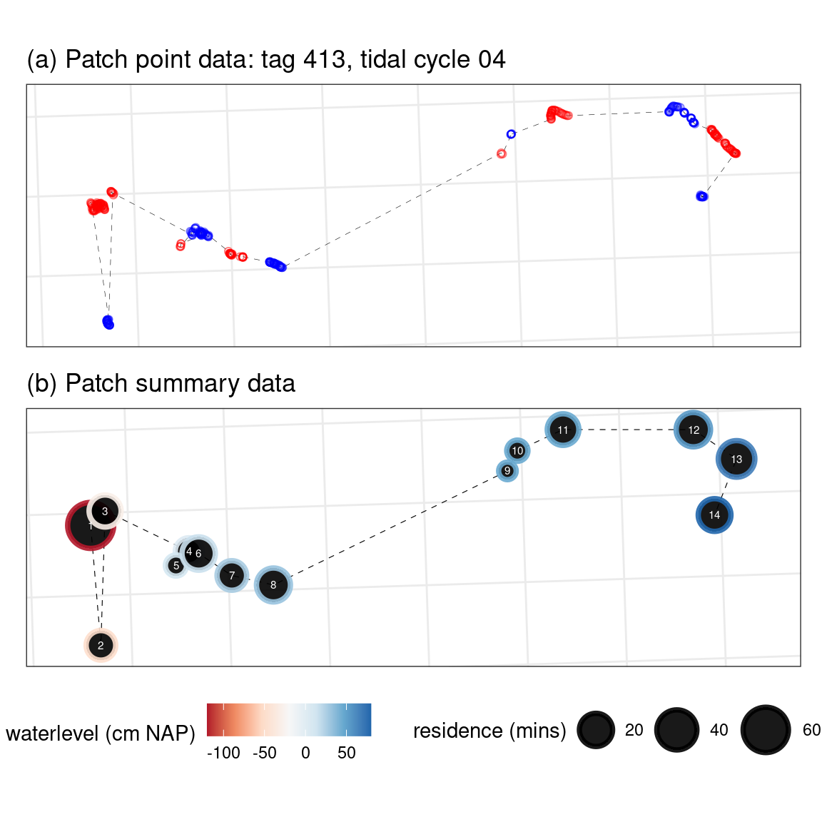
This vignette shows the basics of using watlastools. It is a work in progress. watlastools has two main purposes: accessing and cleaning data, and identifying residence patches from the data. Only the latter is covered here.
library(watlastools)
Making residence patches
Residence patches are the end goal of the watlastools workflow. They are a conveninent way of synthesising large amounts of tracking data into a few spatially explicit units that have a set of associated (mean) coordinates, as well as ecologically relevant coordinates such as duration.
Begin by reading in the data.
# read data and see leading lines
library(data.table)
data <- fread("vignette_data/413_004_revisit.csv")

head(data)
#>           x       y coordIdx            temp_time                          ts
#> 1: 646876.3 5903885        1 2018-08-12T13:30:00Z 2018-08-12T13:25:29.634667Z
#> 2: 646810.2 5904035        2 2018-08-12T13:30:00Z    2018-08-12T13:25:46.634Z
#> 3: 646929.2 5903835        3 2018-08-12T13:30:00Z    2018-08-12T13:32:37.615Z
#> 4: 646877.9 5903939        4 2018-08-12T13:30:00Z 2018-08-12T13:32:57.114500Z
#> 5: 646930.5 5903887        5 2018-08-12T13:40:00Z    2018-08-12T13:36:25.605Z
#> 6: 646972.9 5903816        6 2018-08-12T13:40:00Z 2018-08-12T13:36:57.603333Z
#>          time  id posID    X_raw   Y_raw NBS     VARX     VARY     COVXY
#> 1: 1534080330 413   3.0 646876.3 5903885   3 1409.000 6058.883 -2880.460
#> 2: 1534080360 413   5.0 646810.2 5904035   3 2338.890 9407.620 -4618.900
#> 3: 1534080750 413   8.0 646929.2 5903835   3  609.179 2814.890 -1295.480
#> 4: 1534080780 413   9.5 646877.9 5903939   3 1136.403 4910.655 -2330.560
#> 5: 1534080990 413  11.0 646930.5 5903887   3 1402.250 6461.530 -2989.980
#> 6: 1534081020 413  13.0 646972.9 5903816   3 1086.319 5678.337 -2437.807
#>          SD tide_number tidaltime waterlevel    resTime        fpt revisits
#> 1: 41.21546           4  335.4939       -106 0.08615906 0.08615906        1
#> 2: 50.08702           4  335.7772       -106 1.55416984 1.55416984        1
#> 3: 28.86363           4  342.6269       -106 5.72246712 1.60784093        2
#> 4: 36.92465           4  342.9519       -106 2.49882594 2.49882594        1
#> 5: 43.40300           4  346.4268       -113 2.68004833 2.68004833        1
#> 6: 43.25045           4  346.9601       -113 7.87090615 0.09736257        2
Now make residence patches after inferring residence from gaps in the data.
# run the three main functions on the data
# first infer residence
temp_data <- wat_infer_residence(data = data,
                                 inf_patch_time_diff = 30,
                                 inf_patch_spat_diff = 100)

# classify residence points
temp_data <- wat_classify_points(data = temp_data,
                                 lim_res_time = 2)

# make residence patches with sensible parameters
patches <- wat_make_res_patch(data = temp_data,
                              buffer_radius = 10,
                              lim_spat_indep = 100,
                              lim_time_indep = 30,
                              lim_rest_indep = 30,
                              min_fixes = 3)
Getting data from patches
Get and view the different kinds of patch data
Patch summary
The patch summary is a data.table and has no complex (list, sf) column types. The patches can be visualised using ggplot (or anything else).
# get patch summary
patch_summary <- wat_get_patch_summary(res_patch_data = patches,
                                       which_data = "summary")

# get the class of the full object and the column types
class(patch_summary)
#> [1] "data.table" "data.frame"
Patch points
The patch points are the raw points that make up the residence patches.
# get patch points
patch_points <- wat_get_patch_summary(res_patch_data = patches,
                                      which_data = "points")

# get class and column type
class(patch_points)
#> [1] "data.table" "data.frame"
Patch polygons
This should have the added class sf, and the polygons column should have the type sfc_MULTIPOLYGON.
# get patch points
patch_polygons <- wat_get_patch_summary(res_patch_data = patches,
                                      which_data = "spatial")

# get class and column type
class(patch_polygons)
#> [1] "sf"         "data.table" "data.frame"
