Section 2 Processing Egyptian Fruit Bat Tracks
We show the pre-processing pipeline at work on the tracks of three Egyptian fruit bats (Rousettus aegyptiacus), and construct residence patches.
2.1 Prepare libraries
Install the required R libraries that are required from CRAN if not already installed.
2.2 Read bat data
Read the bat data from an SQLite database local file and convert to a plain text csv file.
This data can be found in the “data” folder.
# prepare the connection
con <- dbConnect(
  drv = SQLite(),
  dbname = "data/Three_example_bats.sql"
)

# list the tables
table_name <- dbListTables(con)

# prepare to query all tables
query <- sprintf('select * from \"%s\"', table_name)

# query the database
data <- dbGetQuery(conn = con, statement = query)

# disconnect from database
dbDisconnect(con)
Convert data to csv, and save a local copy in the folder “data”.
2.3 Exploratory Data Analysis Panels: Main Text Figure 1
Here, we make some basic figures for exploratory data analysis shown in Figure 1 of the main text.
Plot the bat data as a sanity check, and inspect it visually for errors.
The plot code is hidden in the rendered copy (PDF) of this supplementary material, but is available in the Rmarkdown file “supplement/06_bat_data.Rmd”.
2.3.1 Heatmap of Locations
Here we demonstrate a basic heatmap of locations, aggregating over all individuals. In this one instance, the plotting code is also shown as a guide for readers, but in general, plotting code is hidden throughout this document.
data_heatmap <- copy(data)
data_heatmap[, c("xround", "yround") := list(
  plyr::round_any(X, 250),
  plyr::round_any(Y, 250)
)]
data_heatmap <- data_heatmap[, .N, by = c("xround", "yround")]
fig_heatmap <-
ggplot(data_heatmap) +
geom_tile(
aes(
xround, yround,
fill = N
),
size = 0.1,
show.legend = F
) +
scale_fill_viridis_c(
option = "A",
direction = -1,
trans = "log10"
) +
theme_void() +
coord_sf(crs = 2039)
ggsave(fig_heatmap,
filename = "supplement/figures/fig_bat_heatmap_raw.png",
dpi = 300,
width = 6, height = 4
)2.3.2 Sampling Intervals
Here, we create the histogram of sampling intervals shown in Figure 1 of the main text. The plotting code is hidden in the PDF version, but available in the source code.
2.3.3 Localisation Error Measured by Systems
Here, we create the histogram of location error (variance in X) (Weiser et al. 2016) shown in Figure 1 of the main text. The plotting code is hidden in the PDF version, but available in the source code.
2.3.4 Plot paths from raw tracking data
Here, we plot the paths of individual bats from the raw tracking data to visually inspect them for errors.
# this figure for the panel in main text figure 1
fig_bat_focus_bad_speed <-
  fig_bat_raw +
  coord_sf(
    crs = 2039,
    xlim = c(253000, NA),
    ylim = c(772000, NA)
  )

# save to supplement figures
ggsave(fig_bat_focus_bad_speed,
  filename = "supplement/figures/fig_bat_focus_bad_speed.png",
  dpi = 300,
  width = 4, height = 6
)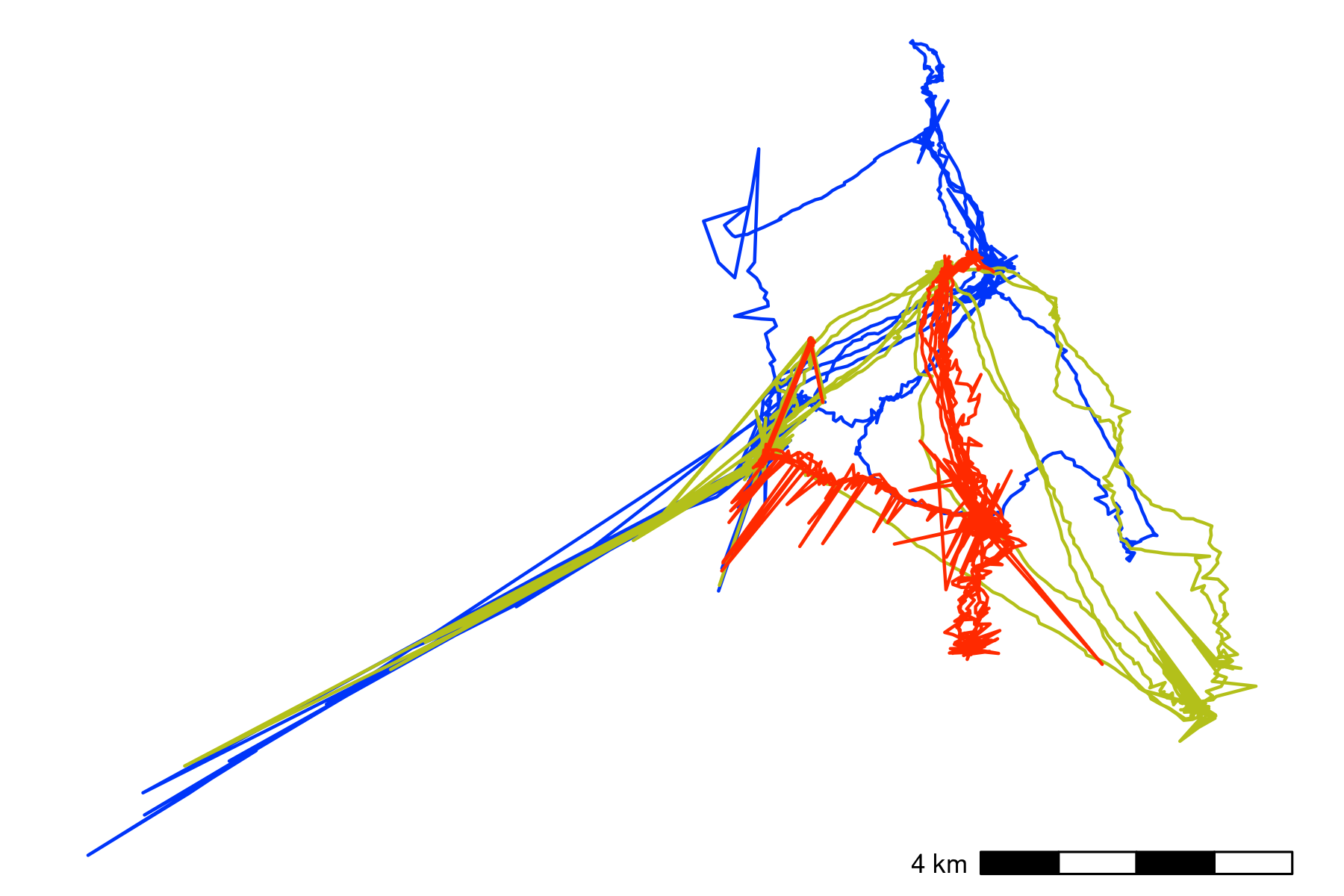
Movement data from three Egyptian fruit bats tracked using the ATLAS system (Rousettus aegyptiacus; (Toledo et al. 2020; Shohami and Nathan 2020)). The bats were tracked in the Hula Valley, Israel (33.1\(^{\circ}\)N, 35.6\(^{\circ}\)E), and we use three nights of tracking (5, 6, and 7 May, 2018), for our demonstration, with an average of 13,370 positions (SD = 2,173; range = 11,195 – 15,542; interval = 8 seconds) per individual. After first plotting the individual tracks, we notice severe distortions, making pre-processing necesary
2.4 Prepare data for filtering
Here we apply a series of simple filters. It is always safer to deal with one individual at a time, so we split the data.table into a list of data.tables to avoid mixups among individuals.
This is a very rudimentary demonstration of the principle behind batch processing — splitting data into smaller, independent subsets, and applying the same steps to each subset.
2.4.1 Prepare data per individual
2.5 Filter by system-generated error attributes
No natural bounds suggest themselves, so instead we proceed to filter by system-generated attributes of error, since point outliers are obviously visible.
We use filter out positions with SD > 20 and positions calculated using only 3 base stations, using the function atl_filter_covariates.
First we calculate the variable SD, which for ATLAS systems is calculated as:
\[SD = \sqrt{{VARX} + {VARY} + 2 \times {COVXY}}\]
# get SD.
# since the data are data.tables, no assignment is necessary
invisible(
  lapply(data_split, function(dt) {
    dt[, SD := sqrt(VARX + VARY + (2 * COVXY))]
  })
)
Then we pass the filters to atl_filter_covariates.
We apply the filter to each individual’s data using an lapply – this separates the data from each individual into a separate data frame, lessening the chances of inter-individual mix-ups.
This is another basic example of the principles behind batch-processing, and could be parallelised using the R package furrr (see https://CRAN.R-project.org/package=furrr).
# filter for SD <= 20
# here, reassignment is necessary as rows are being removed
data_split <- lapply(data_split, function(dt) {
  dt <- atl_filter_covariates(
    data = dt,
    filters = c(
      "SD <= 20",
      "NBS > 3"
    )
  )
})
2.5.1 Sanity check: Plot filtered data
We plot the data to check whether the filtering has improved the data (Fig. 2.2). The plot code is once again hidden in this rendering, but is available in the source code file.
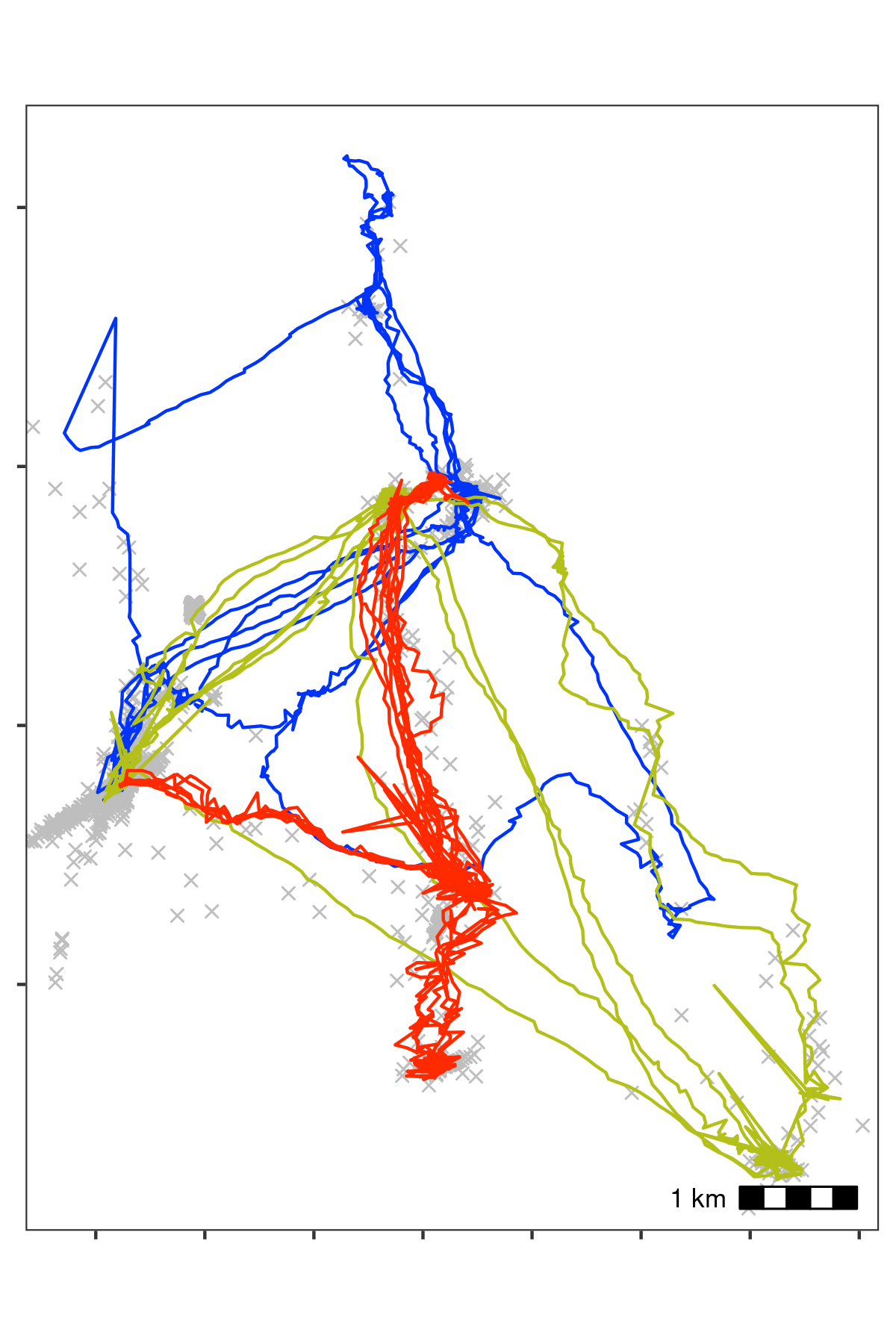
Bat data filtered for large location errors, removing observations with standard deviation \(>\) 20. Grey crosses show data that were removed. Since the number of base stations used in the location process is a good indicator of error (Weiser et al. 2016), we also removed observations calculated using fewer than four base stations. Both steps used the function . This filtering reduced the data to an average of 10,447 positions per individual (78% of the raw data on average). However, some point outliers remain.
2.6 Filter by speed
Some point outliers remain, and could be removed using a speed filter.
First we calculate speeds, using atl_get_speed. We must assign the speed output to a new column in the data.table, which has a special syntax which modifies in place, and is shown below. This syntax is a feature of the data.table package, not strictly of atlastools (Dowle and Srinivasan 2020).
# get speeds as with SD, no reassignment required for columns
invisible(
  lapply(data_split, function(dt) {

    # first process time to seconds
    # assign to a new column
    dt[, time := floor(TIME / 1000)]

    dt[, `:=`(
      speed_in = atl_get_speed(dt,
        x = "X", y = "Y",
        time = "time",
        type = "in"
      ),
      speed_out = atl_get_speed(dt,
        x = "X", y = "Y",
        time = "time",
        type = "out"
      )
    )]
  })
)
Now filter for speeds > 20 m/s (around 70 km/h), passing the predicate (a statement return TRUE or FALSE) to atl_filter_covariates. First, we remove positions which have NA for their speed_in (the first position) and their speed_out (last position).
# filter speeds
# reassignment is required here
data_split <- lapply(data_split, function(dt) {
  dt <- na.omit(dt, cols = c("speed_in", "speed_out"))

  dt <- atl_filter_covariates(
    data = dt,
    filters = c(
      "speed_in <= 20",
      "speed_out <= 20"
    )
  )
})
2.6.1 Sanity check: Plot speed filtered data
The speed filtered data is now inspected for errors (Fig. 2.3). The plot code is once again hidden.
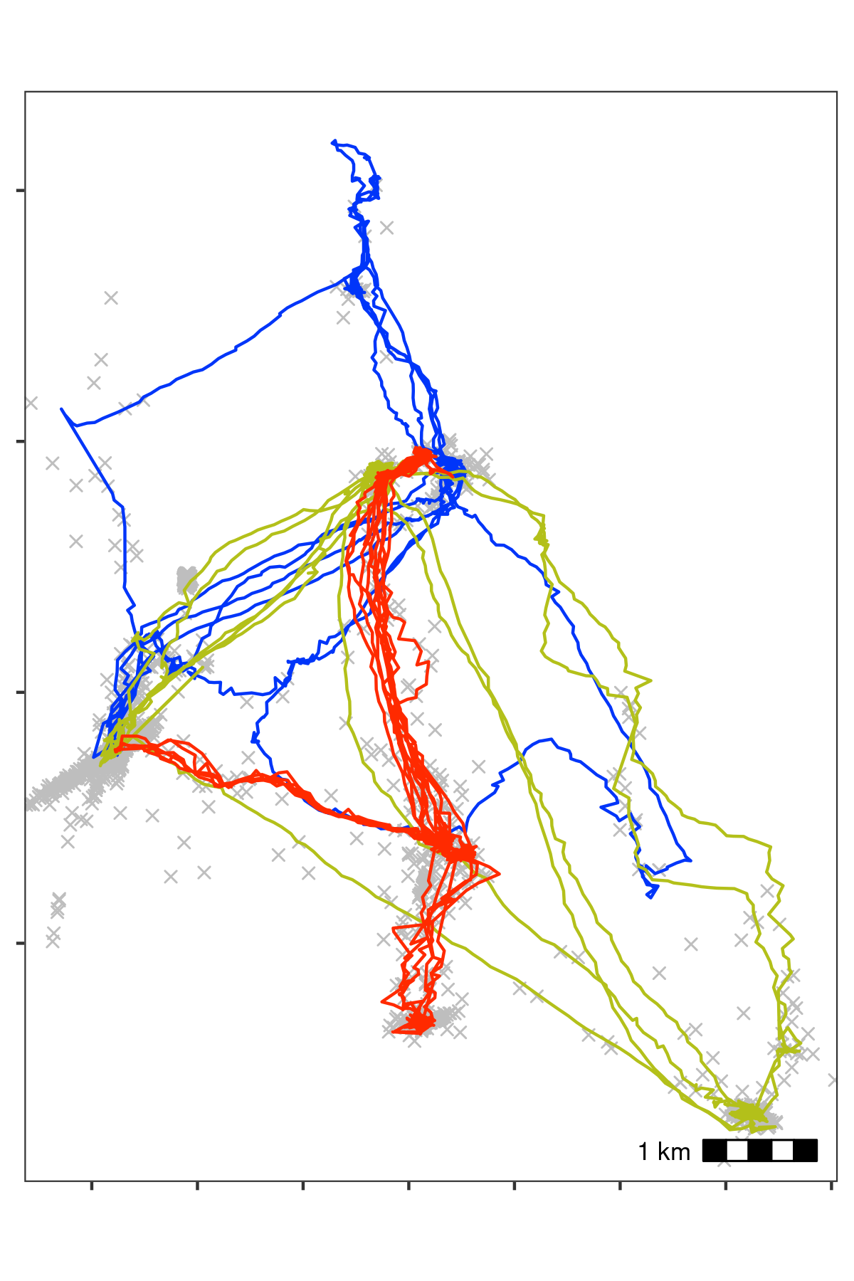
Bat data with unrealistic speeds removed. Notice, compared with the previous figure, that spikes of unrealistic movement in all three tracks have been removed. Grey crosses show data that were removed. We calculated the incoming and outgoing speed of each position using atl_get_speed, and filtered out positions with speeds > 20 m/s using atl_filter_covariates, leaving 10,337 positions per individual on average (98% from the previous step).
2.7 Median smoothing
The quality of the data is relatively high, and a median smooth is not strictly necessary. We demonstrate the application of a 5 point median smooth to the data nonetheless (Fig. 2.4).
Since the median smoothing function atl_median_smooth modifies in place, we first make a copy of the data, using data.table’s copy function.
No reassignment is required, in this case. The lapply function allows arguments to atl_median_smooth to be passed within lapply itself.
In this case, the same moving window \(K\) is applied to all individuals, but modifying this code to use the multivariate version Map allows different \(K\) to be used for different individuals. This is a programming matter, and is not covered here further.
# since the function modifies in place, we shall make a copy
data_smooth <- copy(data_split)

# split the data again
data_smooth <- split(data_smooth, by = "TAG")
# apply the median smooth to each list element
# no reassignment is required as THE FUNCTION MODIFIES IN PLACE!
invisible(
# the function arguments to atl_median_smooth
# can be passed directly in lapply
lapply(
X = data_smooth,
FUN = atl_median_smooth,
time = "time", moving_window = 5
)
)2.7.1 Sanity check: Plot smoothed data
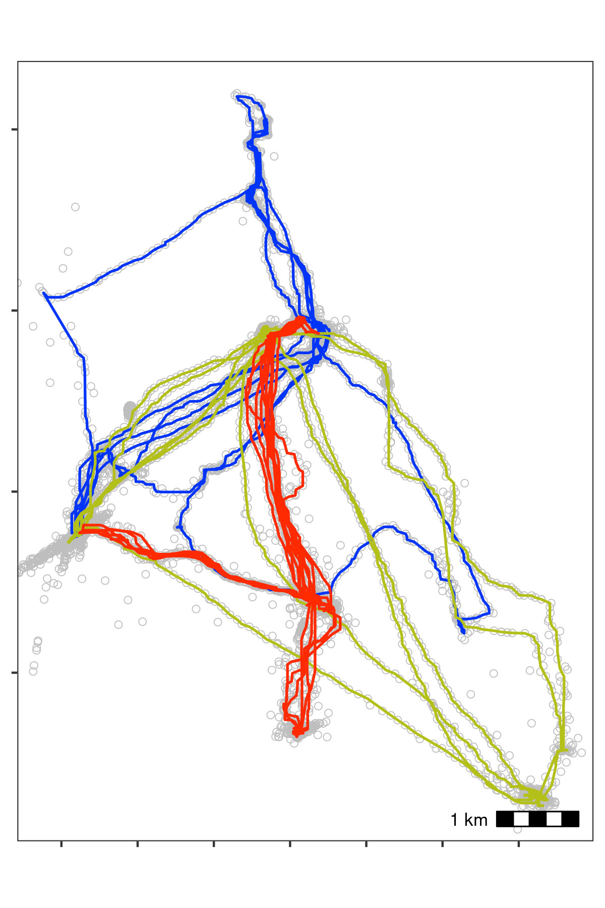
Bat data after applying a median smooth with a moving window \(K\) = 5. Grey circles show data prior to smoothing. The smoothing step did not discard any data.
2.8 Making residence patches
2.8.1 Calculating residence time
First, the data is put through the recurse package to get residence time (Bracis, Bildstein, and Mueller 2018).
We calculated residence time, but since bats may revisit the same features, we want to prevent confusion between frequent revisits and prolonged residence.
For this, we stop summing residence times within \(Z\) metres of a location if the animal exited the area for one hour or more. The value of \(Z\) (radius, in recurse parameter terms) was chosen as 50m.
This step is relatively complicated and is only required for individuals which frequently return to the same location, or pass over the same areas repeatedly, and for which revisits (cumulative time spent) may be confused for residence time in a single visit.
While a simpler implementation using total residence time divided by the number of revisits is also possible, this does assume that each revisit had the same residence time.
# get residence times
data_residence <- lapply(data_smooth, function(dt) {

  # do basic recurse -- refer to Bracis et al. (2018) Ecography
  dt_recurse <- getRecursions(
    x = dt[, c("X", "Y", "time", "TAG")],
    radius = 50,
    timeunits = "mins"
  )

  # get revisit stats column provided as recurse output
  dt_recurse <- setDT(
    dt_recurse[["revisitStats"]]
  )

  # count long absences from the each position
  dt_recurse[, timeSinceLastVisit :=
    ifelse(is.na(timeSinceLastVisit), -Inf, timeSinceLastVisit)]
  dt_recurse[, longAbsenceCounter := cumsum(timeSinceLastVisit > 5),
    by = .(coordIdx)
  ]

  # filter data to exclude revisits after the first long absence of 60 mins
  dt_recurse <- dt_recurse[longAbsenceCounter < 1, ]

  # calculate the residence time as the sum of times inside
  # before the first 'long absence'
  # also calculate the First Passage Time and the number of revisits
  dt_recurse <- dt_recurse[, list(
    resTime = sum(timeInside),
    fpt = first(timeInside),
    revisits = max(visitIdx)
  ),
  by = .(coordIdx, x, y)
  ]

  # prepare to merge existing data with recursion data
  dt[, coordIdx := seq(nrow(dt))]

  # merge the revised recursion analysis data with the tracking data
  dt <- merge(dt,
    dt_recurse[, c("coordIdx", "resTime")],
    by = c("coordIdx")
  )

  # ensure the data are ordered in ascending order of time
  setorderv(dt, "time")

  # print message when done
  message(sprintf("TAG %s residence times done", unique(dt$TAG)))

  # return the dataframe
  dt
})
We bind the data together and assign a human readable timestamp column.
2.8.2 Movements away from the roost
To focus on night-time bat foraging around fruit trees, we shall filter data both on the timestamps, to select night-time positions, and on the locations, to select positions > 1 km away from the roost-cave at Har Gershom (see main text Fig. 8).
Combining these two filters allows us to exclude bat positions at the roost-cave that may be due to individual-differences in bats’ departure or return times to and from their foraging areas.
# read in roosts and select the Har Gershom roost
roosts <- fread("data/Roosts.csv")
setnames(roosts, "Species", "roost_name")
roosts <- roosts[roost_name == "Har Gershom"]

# define a simple distance function that is vectorised
get_distance_adhoc <- function(x1, y1, x2, y2) {
  sqrt(((x2 - x1)^2) + ((y2 - y1)^2))
}

# calculate distance to roost cave at Har Gershom
data_residence[, distance_roost := get_distance_adhoc(
  x1 = roosts$X,
  x2 = data_residence$X,
  y1 = roosts$Y,
  y2 = data_residence$Y
)]
Users should plot the data to examine the effect of applying filters — this code is shown, but the figure is hidden for brevity.
# plot for sanity check --- this plot is not shown
fig_roost_exclude <-
  ggplot(data_residence) +
  geom_point(
    aes(X, Y, col = distance_roost)
  ) +
  geom_point(
    data = roosts,
    aes(X, Y),
    shape = 21, size = 4,
    fill = "blue",
    alpha = 0.5
  ) +
  scale_colour_viridis_c(
    option = "B", direction = -1,
    trans = "log10",
    breaks = c(1000, 2500, 5000),
    labels = function(x) {
      scales::comma(
        x,
        scale = 0.001, suffix = "km"
      )
    },
    limits = c(1000, NA),
    na.value = "lightblue"
  ) +
  ggspatial::annotation_scale(location = "br") +
  theme_test() +
  theme(
    axis.text = element_blank(),
    axis.title = element_blank(),
    legend.position = "top",
    legend.key.height = unit(2, "mm"),
    legend.title = element_text(vjust = 1)
  ) +
  coord_sf(
    crs = 2039
  ) +
  labs(
    colour = "distance (km)"
  )
We now filter the data to exclude both day-time data, as well as data that is < 1 km from the roost.
2.8.3 Split data by night-id
We assign a night-id to each position, i.e., the night-time spanning two calendar days. We then filter for data with a residence time > 5 minutes, as we expect that a bat stopped at a location for more than 5 minutes is likely to be foraging.
2.8.4 Constructing residence patches
Some preparation is required. First, the function requires columns x, y,
time, and id, which we assign using the data.table syntax. The time column is already present, but the other columns need to be renamed to lower case.
# add an id column
data_residence[, `:=`(
  id = TAG,
  x = X, y = Y
)]

# get mean residence time per id
data_residence[, list(
  mean_residence = mean(resTime),
  sd_residence = sd(resTime)
), by = "TAG"]
#>             TAG mean_residence sd_residence
#> 1: 972001004424          238.4        116.8
#> 2: 972001004449           52.8         33.5
#> 3: 972001004452           53.5         38.5

# get mean residence time for all bats pooled
data_residence[, list(
  mean_residence = mean(resTime),
  sd_residence = sd(resTime)
)]
#>    mean_residence sd_residence
#> 1:            133          123

# average positions per bat after removing transit points
data_residence[, list(.N), by = "TAG"][, list(mean_positions_ = mean(N))]
#>    mean_positions_
#> 1:            5549

# split the data
data_residence <- split(data_residence, by = c("TAG", "night"))
We apply the residence patch method, using the default argument values (lim_spat_indep = 100 (metres), lim_time_indep = 30 (minutes)). We change the buffer_radius to 25 metres (twice the buffer radius is used, so points must be separated by 50m to be independent bouts), and min_fixes = 3.
2.8.5 Getting residence patch data
We extract the residence patch data as spatial sf-MULTIPOLYGON objects.
These are returned as a list and must be converted into a single sf object.
These objects and the raw movement data are shown in Fig. 2.5.
# get data spatials
data_spatials <- lapply(data_patches, atl_patch_summary,
  which_data = "spatial",
  buffer_radius = 25
)

# bind list
data_spatials <- rbindlist(data_spatials)

# convert to sf
library(sf)
data_spatials <- st_sf(data_spatials, sf_column_name = "polygons")

# assign a crs
st_crs(data_spatials) <- st_crs(2039)
2.8.6 Write patch spatial representations
st_write(data_spatials,
  dsn = "data/data_bat_residence_patches.gpkg",
  append = FALSE
)
#> Deleting layer `data_bat_residence_patches' using driver `GPKG'
#> Writing layer `data_bat_residence_patches' to data source
#>   `data/data_bat_residence_patches.gpkg' using driver `GPKG'
#> Writing 45 features with 22 fields and geometry type Multi Polygon.
Write cleaned bat data.
Write patch summary.
2.8.7 Duration at foraging sites
We exclude the first and last patch of each day as being roosting related, and examine how much of the total foraging time (time between the remaining first and last patch) was spent at foraging sites. It follows that the remainder of the time must have been spent in transit, or otherwise not foraging.
# make patch summary a datatable
setDT(patch_summary)

# get mean and sd of duration in patches
patch_summary[, list(
  mean_duration = mean(duration / 60),
  sd_duration = sd(duration / 60)
)]
#>    mean_duration sd_duration
#> 1:            57        62.2

# assign night id
patch_summary[, c("hour", "day") := list(
  data.table::hour(as.POSIXct(time_start, origin = "1970-01-01")),
  data.table::mday(as.POSIXct(time_start, origin = "1970-01-01"))
)]

# get total foraging time
foraging_proportion <- patch_summary[, list(
  time_total_forage = (max(time_end) - min(time_start)) / 60,
  time_forage_site = sum(duration / 60)
),
by = c("id", "night_mean")
]

# get proporion of foraging that is at a foraging site
foraging_proportion[, list(
  mean_foraging_prop = mean(time_forage_site / time_total_forage),
  sd_foraging_prop = sd(time_forage_site / time_total_forage)
)]
#>    mean_foraging_prop sd_foraging_prop
#> 1:              0.838            0.155
2.9 Main text Figure 8
See Fig. 8 in the main text, made with QGIS.

A visual examination of plots of the bats’ residence patches and linear approximations of paths between them showed that though all three bats roosted at the same site, they used distinct areas of the study site over the three nights (a). Bats tended to be resident near fruit trees, which are their main food source, travelling repeatedly between previously visited areas (b, c). However, bats also appeared to spend some time at locations where no fruit trees were recorded, prompting questions about their use of other food sources (b, c). When bats did occur close together, their residence patches barely overlapped, and their paths to and from the broad area of co-occurrence were not similar (c). Constructing residence patches for multiple individuals over multiple activity periods suggests interesting dynamics of within- and between-individual overlap (b, c).
References
Bracis, Chloe, Keith L. Bildstein, and Thomas Mueller. 2018. “Revisitation Analysis Uncovers Spatio-Temporal Patterns in Animal Movement Data.” Ecography 41 (11): 1801–11. https://doi.org/10.1111/ecog.03618.
Dowle, Matt, and Arun Srinivasan. 2020. Data.Table: Extension of ‘data.Frame‘. Manual.
Shohami, David, and Ran Nathan. 2020. “Cognitive Map-Based Navigation in Wild Bats Revealed by a New High-Throughput Tracking System.” Dryad. https://doi.org/10.5061/DRYAD.G4F4QRFN2.
Toledo, Sivan, David Shohami, Ingo Schiffner, Emmanuel Lourie, Yotam Orchan, Yoav Bartan, and Ran Nathan. 2020. “Cognitive MapBased Navigation in Wild Bats Revealed by a New High-Throughput Tracking System.” Science 369 (6500). American Association for the Advancement of Science: 188–93. https://doi.org/10.1126/science.aax6904.
Weiser, Adi Weller, Yotam Orchan, Ran Nathan, Motti Charter, Anthony J. Weiss, and Sivan Toledo. 2016. “Characterizing the Accuracy of a Self-Synchronized Reverse-GPS Wildlife Localization System.” In 2016 15th ACM/IEEE International Conference on Information Processing in Sensor Networks (IPSN), 1–12. https://doi.org/10.1109/IPSN.2016.7460662.