Section 3 Speed and collar temperature

Here we look at the relationship between elephant speed and collar temperature, as well as some other relevant factors that we think might influence elephant movement.

3.1 Load libraries

# load libraries
library(dplyr)
library(purrr)
library(lubridate)
library(readr)

# stats
library(mgcv)

# spatial
library(sf)
library(raster)

# plotting
library(ggplot2)
library(ggthemes)
library(viridis)

# custom funcs
ci = function(x) 1.96*sd(x, na.rm = T)/sqrt(length(x))

3.2 Load data from sources

Load the tracking data and the transformed slope data.

# read in eles as csv
data = read_csv("data/elephant_data.csv")

3.3 Speed and temperature

3.3.1 Run GAMM speed ~ temperature

# make id a factor
data$id = as.factor(data$id)
data$season = as.factor(data$season)

# run a GAMM using the mgcv package
mod.speed = bam(v ~ s(temp, k = 4) + 
  season + 
  woody.density + 
  s(id, bs = "re") + 
  s(hour, bs = "re"), 
  data = data)

# print model summary to file
if(!dir.exists("data/model_output")){
  dir.create("data/model_output")
}

if(file.exists("data/model_output/model_gamm_speed.txt")){
  file.remove("data/model_output/model_gamm_speed.txt")
}

R.utils::captureOutput(summary(mod.speed), 
              file = "data/model_output/model_gamm_speed.txt",
              append = TRUE)

Print the GAMM summary.

cat(readLines("data/model_output/model_gamm_speed.txt"), sep = "\n")

Family: gaussian 
Link function: identity 

Formula:
v ~ s(temp, k = 4) + season + woody.density + s(id, bs = "re") + 
    s(hour, bs = "re")

Parametric coefficients:
               Estimate Std. Error t value Pr(>|t|)    
(Intercept)   252.55538    5.20079   48.56   <2e-16 ***
seasonwet      16.48085    0.86423   19.07   <2e-16 ***
woody.density  -1.60256    0.03278  -48.89   <2e-16 ***
---
Signif. codes:  0 ‘***’ 0.001 ‘**’ 0.01 ‘*’ 0.05 ‘.’ 0.1 ‘ ’ 1

Approximate significance of smooth terms:
           edf Ref.df      F p-value    
s(temp)  2.995      3 4716.1  <2e-16 ***
s(id)   12.890     13  131.2  <2e-16 ***
s(hour)  0.991      1  112.6  <2e-16 ***
---
Signif. codes:  0 ‘***’ 0.001 ‘**’ 0.01 ‘*’ 0.05 ‘.’ 0.1 ‘ ’ 1

R-sq.(adj) =  0.0667   Deviance explained = 6.68%
fREML = 1.9511e+06  Scale est. = 52787     n = 284572

3.3.2 Prepare speed ~ temp plot data

# prepare data for plotting
ele.speed.temp = 
  data %>%
  mutate(v.pred = predict(mod.speed, 
                          newdata = ., scale = "response", 
                          allow.new.levels = T), 
         temp = plyr::round_any(temp,2)) %>%
  ungroup() %>% 
  
  group_by(season, temp) %>%
  
  summarise(v.mean = mean(v), 
            v.sd = sd(v), 
            n.v = length(v), 
            pred.mean = mean(v.pred, na.rm = T), 
            pred.sd=sd(v.pred, na.rm = T), 
            pred.n = length(v.pred)) %>%
  
  mutate(v.ci = qnorm(0.975)*v.sd/sqrt(n.v), 
         ci.pred = qnorm(0.975)*pred.sd/sqrt(pred.n))

3.3.3 Prepare Figure 4 (A): Speed and temperature

# figure for speed and temperature
fig_speed_temp =
  ele.speed.temp %>% 
  filter(temp %in% 10:40) %>%
  ggplot()+
    
  geom_rangeframe(data = data_frame(x=c(10,40), y = c(0.15,0.6)),aes(x,y))+
  geom_smooth(aes(x = temp, y = pred.mean*2/1e3, 
                  col = season, fill = season, lty = season), 
              alpha = 0.2, lwd = 0.5)+
  geom_pointrange(aes(x = temp, y = v.mean*2/1e3, 
                      ymin = (v.mean-v.ci)*2/1e3, ymax = (v.mean+v.ci)*2/1e3, 
                      col = season, shape = season), 
                  fill = "white", size = 0.4, stroke =0.7, lty = 1, 
                  position = position_dodge(width = 0.3))+

  scale_fill_brewer(palette = "Set1")+
  scale_color_brewer(palette = "Set1")+
  scale_shape_manual(values=c(21,24))+
  scale_linetype_manual(values=c("dashed","solid"))+
  
  theme_few()+
  theme(panel.border = element_blank(),
        legend.position = "none")+
  coord_cartesian(ylim=c(0.15,0.6))+
  scale_y_continuous(breaks = seq(.15,.6,.15))+
  labs(x = "Collar temperature (°C)", y = "Speed (km/h)",
            col = "Season", fill = "Season", title="(a)")

3.3.4 Prepare data for speed ~ woodland plot

# prepare data
ele.speed.wood = 
  as_data_frame(data) %>% 
  mutate(v.pred = predict(mod.speed, 
    newdata = ., scale = "response", allow.new.levels = T)) %>%  
  
  dplyr::select(woody.density, v, v.pred, season) %>% 
  mutate(v2 = v*2/1e3, 
    v.pred2 = v.pred*2/1e3) %>% 
  
  dplyr::select(-v, -v.pred) %>% 
  
  tidyr::gather(var, value, -woody.density, -season) %>% 
  group_by(season, wood = plyr::round_any(woody.density, 5),var) %>%
  
  summarise_at(vars(value), list(mean=mean, sd=sd, length=length)) %>% 
  mutate(ci = 1.96*sd/sqrt(length))

3.3.5 Prepare Figure 4 (B): Speed and woody cover

#review figs: speed vs slope, speed vs woody density
fig_speed_wood = ggplot()+
  geom_smooth(data = ele.speed.wood %>% filter(var == "v.pred2"), 
              aes(x = wood, y = mean, col = season, fill = season, lty = season), 
              alpha = 0.2, size = 0.3)+
  
  geom_pointrange(data = ele.speed.wood %>% filter(var == "v2"), 
                  aes(x = wood, ymin = mean-ci, ymax = mean+ci, y = mean, 
                      col = season, shape = season), 
                  fill = "white", position = position_dodge(width = 0.3), 
                  size = 0.4, stroke = 0.7)+
  
  geom_rangeframe(data = data_frame(x=c(0,80),y=c(0.15,0.6)), aes(x,y))+
  
  #facet_wrap(~var_name, scales = "free_x")+
  
  scale_color_brewer(palette = "Set1")+
  scale_fill_brewer(palette = "Set1")+
  scale_linetype_manual(values=c(2,1))+
  scale_shape_manual(values= c(21,24))+
  
  theme_few()+
  theme(panel.border = element_blank(),
        legend.position = "none")+
  labs(x = "Woody cover (%)", y = "Speed (km/h)", title = "(b)")+
  
  scale_x_continuous(breaks = seq(0, 80, 20))+
  scale_y_continuous(breaks = c(.15,.3,.45,.6), limits = c(NA, .6))+
  coord_cartesian(ylim=c(.15,.6))

3.4 Figure 4: Speed and temperature and woody cover

half = 85/25.4; full = 180/25.4

# export fig for temp measures
library(gridExtra)

figure_04_speed = grid.arrange(fig_speed_temp, fig_speed_wood, nrow = 1)

ggsave(figure_04_speed,
       filename = "figs/figure_04_speed.pdf",
       height = half, width = full)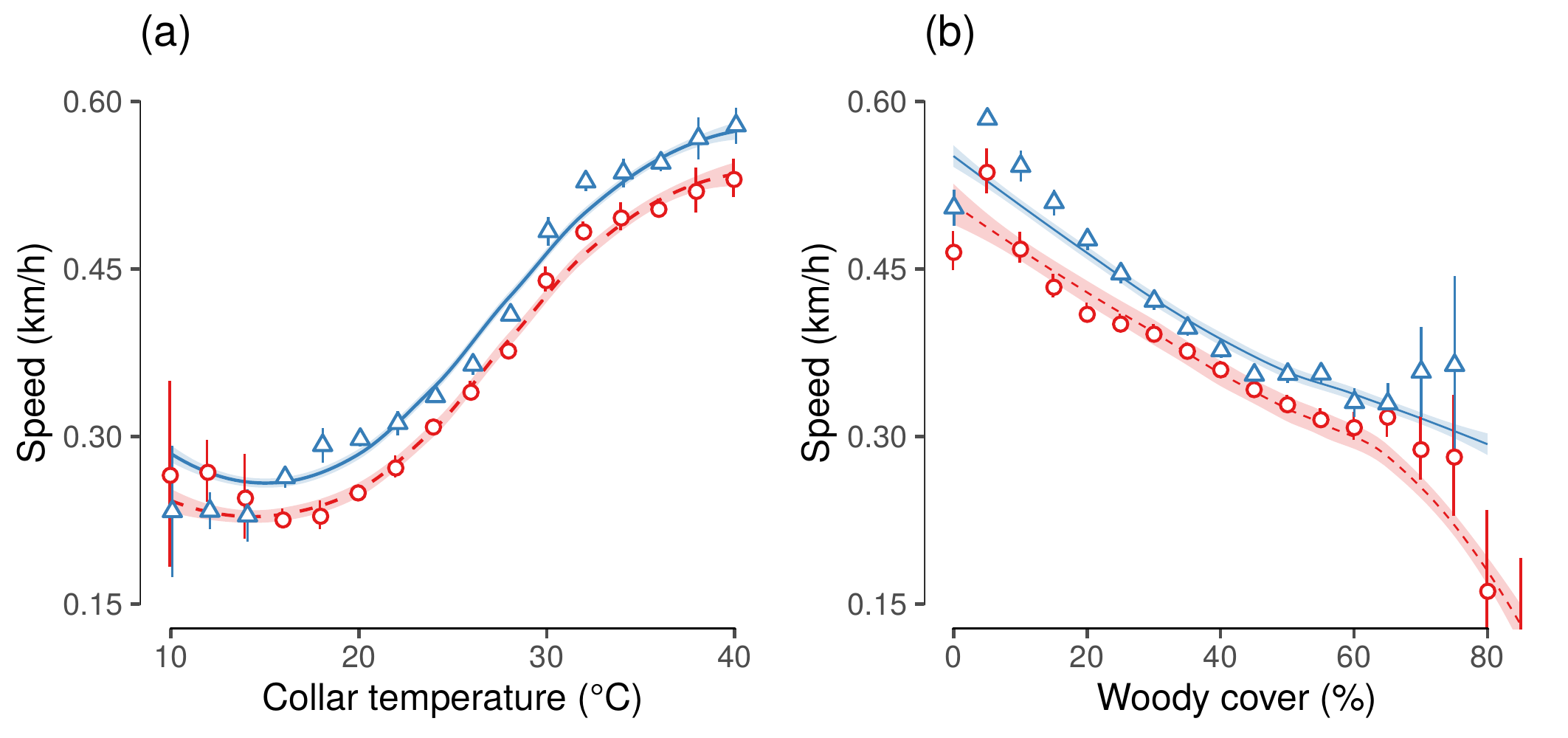

library(magick)
fig04 = magick::image_read_pdf("figs/figure_04_speed.pdf")
fig04

(#fig:show_figure_04)Speed of elephant movement in relation to (a) collar temperature (at 2 ◦ C intervals) and (b) % woody cover (at 5 unit intervals) in the dry (red circles) and wet season (blue triangles). GAMM fit (lines) and 95% confidence intervals (vertical line ranges and shaded areas) are shown for each season separately.