Section 7 Checking Temporal Sampling Frequency

How often are checklists recorded in each grid cell?

7.1 Load libraries

# load libraries
library(tidyverse)
library(sf)

# for plotting
library(ggplot2)
library(colorspace)
library(scico)
library(ggthemes)
library(ggspatial)
library(patchwork)

7.2 Load checklist data

Here we load filtered checklist data and convert to UTM 43N coordinates.

# load checklist data
load("data/01_data_prelim_processing.rdata")

# get checklists
data <- distinct(
  dataGrouped, sampling_event_identifier, observation_date,
  longitude, latitude
)

# remove old data
rm(dataGrouped)

# transform to UTM 43N
data <- st_as_sf(data, coords = c("longitude", "latitude"), crs = 4326)
data <- st_transform(data, crs = 32643)

# get coordinates and bind to data
data <- cbind(
  st_drop_geometry(data),
  st_coordinates(data)
)

# bin to 1000m
data <- mutate(data,
  X = plyr::round_any(X, 2500),
  Y = plyr::round_any(Y, 2500)
)

7.3 Get time differences per grid cell

# get time differences in days
data <- mutate(data, observation_date = as.POSIXct(observation_date))
data <- nest(data, data = c("sampling_event_identifier", "observation_date"))

# map over data
data <- mutate(data,
  lag_metrics = lapply(data, function(df) {
    df <- arrange(df, observation_date)

    lag <- as.numeric(diff(df$observation_date, na.rm = TRUE) / (24 * 3600))

    data <- tibble(
      mean_lag = mean(lag, na.rm = TRUE),
      median_lag = median(lag, na.rm = TRUE),
      sd_lag = sd(lag, na.rm = TRUE),
      n_chk = nrow(df)
    )

    data
  })
)

# unnest lag metrics
data_lag <- select(data, -data)
data_lag <- unnest(data_lag, cols = "lag_metrics")

# set the mean and median to infinity if nchk is 1
data_lag <- mutate(data_lag,
  mean_lag = ifelse(n_chk == 1, Inf, mean_lag),
  median_lag = ifelse(n_chk == 1, Inf, median_lag),
  sd_lag = ifelse(n_chk == 1, Inf, sd_lag)
)

# set all 0 to 1
data_lag <- mutate(data_lag,
  mean_lag = mean_lag + 1,
  median_lag = median_lag + 1
)
# melt data by tile
# data_lag = pivot_longer(data_lag, cols = c("mean_lag", "median_lag", "sd_lag"))

7.4 Time Since Previous Checklist

7.4.1 Get aux data

# hills data
wg <- st_read("data/spatial/hillsShapefile/Nil_Ana_Pal.shp") %>%
  st_transform(32643)

roads <- st_read("data/spatial/roads_studysite_2019/roads_studysite_2019.shp") %>%
  st_transform(32643)

# add land
library(rnaturalearth)
land <- ne_countries(
  scale = 50, type = "countries", continent = "asia",
  country = "india",
  returnclass = c("sf")
) %>%
  st_transform(32643)

bbox <- st_bbox(wg)

7.4.2 Histogram of lags

Figure code hidden in HTML and PDF versions.

# get lags
data <- mutate(data,
  lag_hist = lapply(data, function(df) {
    df <- arrange(df, observation_date)

    lag <- as.numeric(diff(df$observation_date, na.rm = TRUE) / (24 * 3600))

    data <- tibble(
      lag = lag + 1,
      index = seq(lag)
    )

    data
  })
)

# unnest lags
data_hist <- select(data, X, Y, lag_hist) %>%
  unnest(cols = "lag_hist")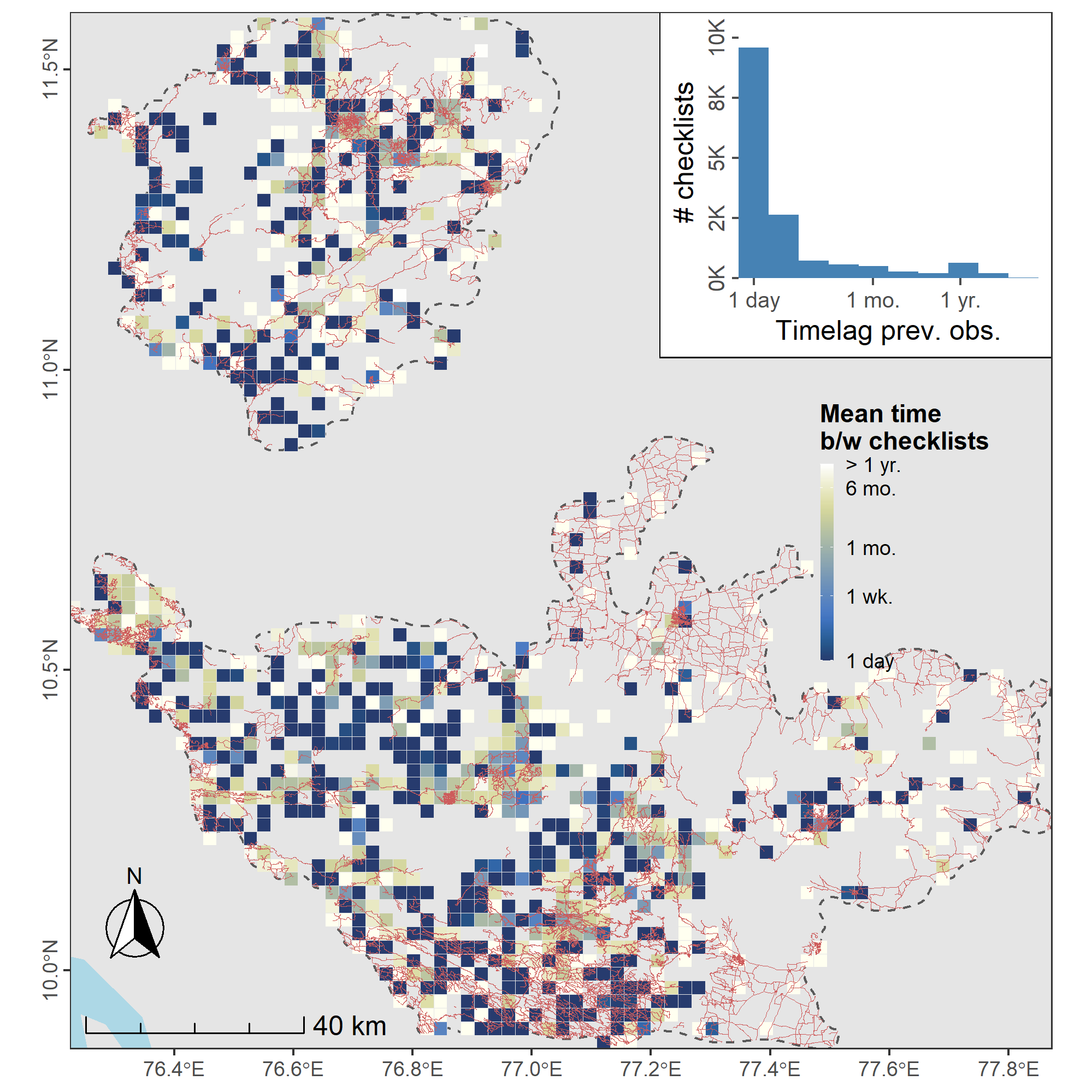

Most sites are resurveyed at least once, but some are visited much more frequently than others. There does not appear to be a link between roads and visit frequency. eBird checklists are also strongly clustered in time, with some of the most sampled areas over the study period visited at intervals of > 1 week, and with some less intensively sampled areas visited frequently, at intervals of < 1 week. Overall, the majority of checklists are reported only a day after the previous checklist at that location (see inset).

7.5 Main Text Figure 3

Combining figures for spatial and temporal clustering into main text figure 3. This overall figure is not shown here, see main text.

# load spatial bias figure
load("data/fig_checklists_grid.Rds")

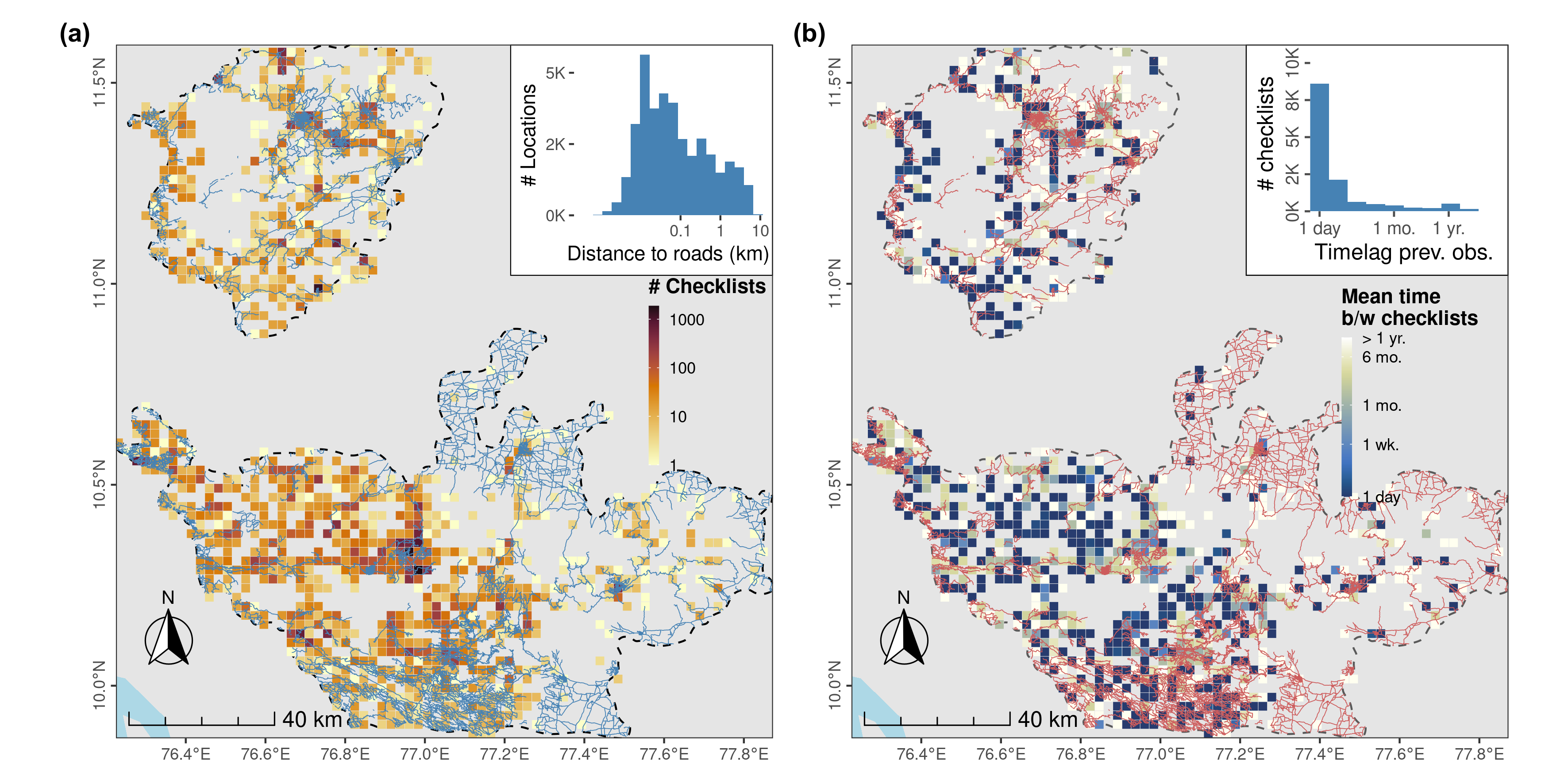
Distribution of sampling effort in the form of eBird checklists in the Nilgiri and Anamalai Hills between 2013 and 2021. (a) Sampling effort across the Nilgiri and Anamalai Hills, in the form of eBird checklists reported by birdwatchers, mostly takes place along roads, with the majority of checklists located <1 km from a roadway (see distribution in inset), and therefore, only about 300m, on average, from the location of another checklist. (b) eBird checklists are also strongly clustered in time, with some of the most sampled areas over the study period visited at intervals of > 1 week, and with some less intensively sampled areas visited frequently, at intervals of < 1 week. Overall, most checklists are reported only a day after the previous checklist at that location (see inset). Both spatial and temporal clustering make data thinning necessary. Both panels show counts or mean intervals in a 2.5km grid cell; the study area is bounded by a dashed line, and roads within it are shown as (a) blue or (b) red lines.

7.6 Checklists per Month

We counted the checklists per month, pooled over years, to determine how sampling effort varies over the year.

# get two week period by date
data <- select(data, X, Y, data)

# unnest
data <- unnest(data, cols = "data")

# get fortnight
library(lubridate)
data <- mutate(data,
  week = week(observation_date),
  week = plyr::round_any(week, 2),
  year = year(observation_date),
  month = month(observation_date)
)

# count checklists per fortnight
data_count <- count(data, month, year)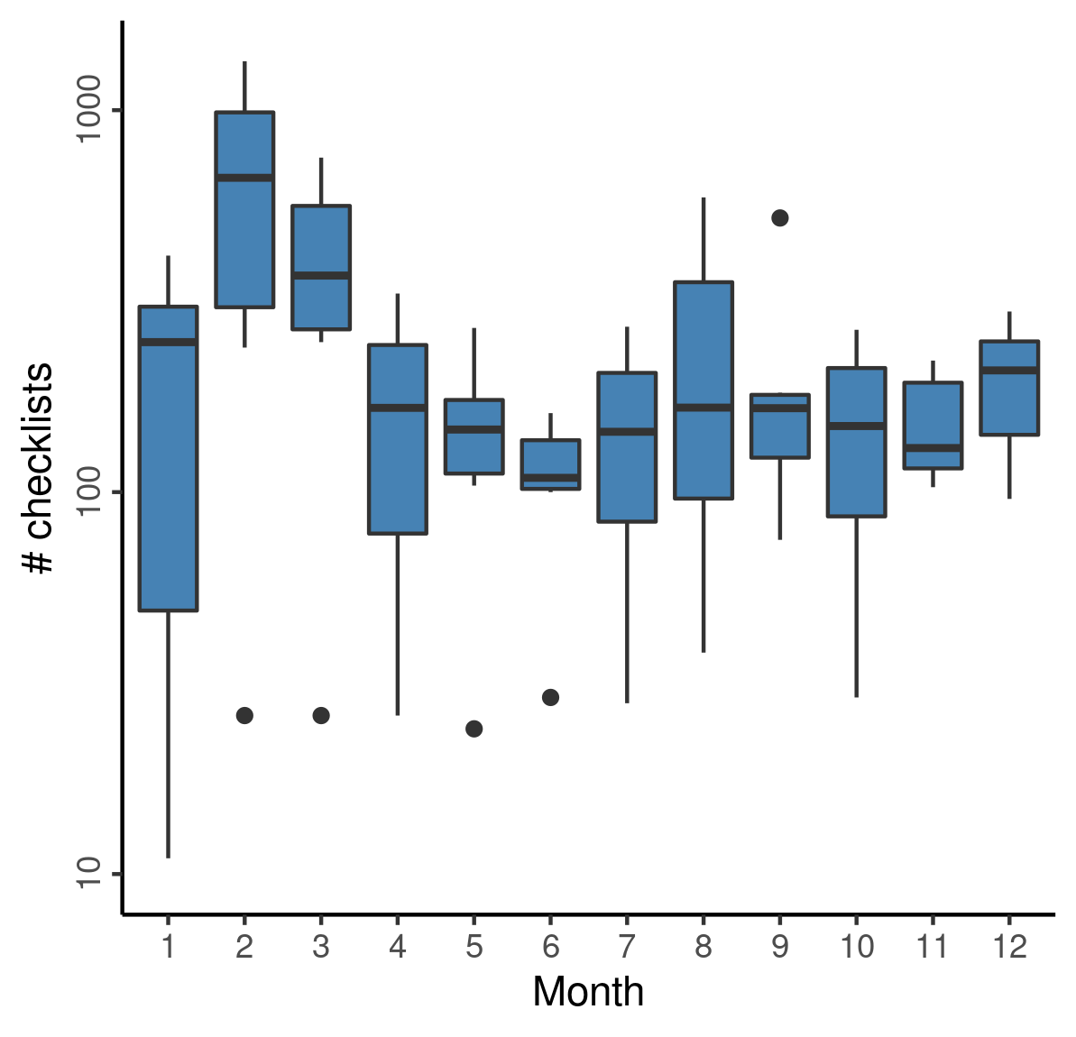

Observations peak in the early months of the year, and decline towards the rainy months, slowly increasing until the following winter.