Section 10 Visualizing Occupancy Predictor Effects

In this section, we will visualize the magnitude and direction of species-specific probability of occupancy.

10.1 Prepare libraries

# to load data
library(readxl)

# to handle data
library(dplyr)
library(readr)
library(forcats)
library(tidyr)
library(purrr)
library(stringr)
# library(data.table)

# to wrangle models
source("R/fun_model_estimate_collection.r")
source("R/fun_make_resp_data.r")

# nice tables
library(knitr)
library(kableExtra)

# plotting
library(ggplot2)
library(patchwork)
source("R/fun_plot_interaction.r")

10.2 Load species list

# list of species
# Removing species after running a chi-square goodness of fit test
species <- read_csv("data/species_list.csv") %>%
  filter(!scientific_name %in% c(
      "Treron affinis", "Prinia hodgsonii", "Pellorneum ruficeps",
      "Hypothymis azurea","Dendrocitta leucogastra","Chalcophaps indica",
      "Rubigula gularis",  "Muscicapa dauurica", "Geokichla citrina", 
      "Chrysocolaptes guttacristatus","Terpsiphone paradisi","Orthotomus sutorius",
      "Oriolus kundoo", "Dicrurus aeneus", "Cyornis tickelliae",
      "Copsychus fulicatus", "Oriolus xanthornus", "Alcippe poioicephala",
      "Ficedula nigrorufa","Dendrocitta vagabunda", "Dicrurus paradiseus",
      "Ocyceros griseus", "Psilopogon viridis", "Psittacula cyanocephala"))

list_of_species <- as.character(species$scientific_name)

10.3 Show AIC weight importance

To get cumulative AIC weights, we first obtained a measure of relative importance of climatic and landscape predictors by calculating cumulative variable importance scores. These scores were calculated by obtaining the sum of model weights (AIC weights) across all models (including the top models) for each predictor across all species. We then calculated the mean cumulative variable importance score and a standard deviation for each predictor (Burnham and Anderson 2002).

10.3.1 Read in AIC weight data

# which files to read
file_names <- c("data/results/lc-clim-imp.xlsx")

# read in sheets by species
model_imp <- map(file_names, function(f) {
  md_list <- map(list_of_species, function(sn) {

    # some sheets are not found

    tryCatch(
      {
        readxl::read_excel(f, sheet = sn) %>%
          `colnames<-`(c("predictor", "AIC_weight")) %>%
          filter(str_detect(predictor, "psi")) %>%
          mutate(
            predictor = stringr::str_extract(predictor,
              pattern = stringr::regex("\\((.*?)\\)")
            ),
            predictor = stringr::str_replace_all(predictor, "[//(//)]", ""),
            predictor = stringr::str_remove(predictor, "\\.y")
          )
      },
      error = function(e) {
        message(as.character(e))
      }
    )
  })
  names(md_list) <- list_of_species

  return(md_list)
})

10.3.2 Prepare cumulative AIC weight data

# bind rows
model_imp <- map(model_imp, bind_rows) %>%
  bind_rows() 

# convert to numeric
model_imp$AIC_weight <- as.numeric(model_imp$AIC_weight)

# Let's get a summary of cumulative variable importance
model_imp <- group_by(model_imp, predictor) %>%
  summarise(
    mean_AIC = mean(AIC_weight),
    sd_AIC = sd(AIC_weight),
    min_AIC = min(AIC_weight),
    max_AIC = max(AIC_weight),
    med_AIC = median(AIC_weight)
  )

# write to file
write_csv(model_imp, "data/results/cumulative_AIC_weights.csv")

Read data back in.

# read data and make factor
model_imp <- read_csv("data/results/cumulative_AIC_weights.csv")
model_imp$predictor <- as_factor(model_imp$predictor)

# make nice names
predictor_name <- tibble(
  predictor = levels(model_imp$predictor),
  pred_name = c(
    "Precipitation seasonality",
    "Temperature seasonality",
    "% Evergreen Forest", "% Deciduous Forest",
    "% Mixed/Degraded Forest", "% Agriculture/Settlements",
    "% Grassland", "% Plantations", "% Water Bodies"
  )
)

# rename predictor
model_imp <- left_join(model_imp, predictor_name)

Prepare figure for cumulative AIC weight. Figure code is hidden in versions rendered as HTML and PDF.

10.4 Prepare model coefficient data

For each species, we examined those models which had ΔAICc < 4, as these top models were considered to explain a large proportion of the association between the species-specific probability of occupancy and environmental drivers (Burnham, Anderson, and Huyvaert 2011; Elsen et al. 2017). Using these restricted model sets for each species; we created a model-averaged coefficient estimate for each predictor and assessed its direction and significance (Bartoń 2020). We considered a predictor to be significantly associated with occupancy if the range of the 95% confidence interval around the model-averaged coefficient did not contain zero.

file_read <- c("data/results/lc-clim-modelEst.xlsx")

# read data as list column
model_est <- map(list_of_species, function(sn) {
  tryCatch(
    {
      readxl::read_excel(file_read, sheet = sn) %>%
        rename(predictor = "...1") %>%
        filter(str_detect(predictor, "psi")) %>%
        mutate(
          predictor = stringr::str_extract(predictor,
            pattern = stringr::regex("\\((.*?)\\)")
          ),
          predictor = stringr::str_replace_all(predictor, "[//(//)]", ""),
          predictor = stringr::str_remove(predictor, "\\.y")
        )
    },
    error = function(e) {
      message(as.character(e))
    }
  )
})
# assign names
names(model_est) <- list_of_species

# prepare model data
model_data <- tibble(
  scientific_name = list_of_species
)

# remove null data
model_est <- keep(model_est, .p = function(x) !is.null(x))

# rename model data components and separate predictors
names <- c(
  "predictor", "coefficient", "se", "ci_lower",
  "ci_higher", "z_value", "p_value"
)

# get data for plotting:
model_est <- map(model_est, function(df) {
  colnames(df) <- names
  # df <- separate_interaction_terms(df)
  # df <- make_response_data(df)
  return(df)
})

# add names and scales
model_est <- imap(model_est, function(.x, .y) {
  mutate(.x, scientific_name = .y)
})

# remove modulators
model_est <- bind_rows(model_est) %>%
  dplyr::select(-matches("modulator"))

# join data to species name
model_data <- model_data %>%
  left_join(model_est)

# Keep only those predictors whose p-values are significant:
model_data <- model_data %>%
  filter(p_value < 0.05) %>%
  filter(predictor != "Int")

Export predictor effects.

# get predictor effect data
data_predictor_effect <- distinct(
  model_data,
  scientific_name,
  se,
  predictor, coefficient
)

# write to file
write_csv(data_predictor_effect, "data/results/data_predictor_effect.csv")

Export model data.

model_data_to_file <- model_data %>%
  dplyr::select(
    predictor,
    scientific_name
  )

# remove .y
model_data_to_file <- model_data_to_file %>%
  mutate(predictor = str_remove(predictor, "\\.y"))

write_csv(
  model_data_to_file,
  "data/results/data_occupancy_predictors.csv"
)

Read in data after clearing R session.

# first merge species trait data with significant predictor
species_trait <- read.csv("data/species-trait-dat.csv")
sig_predictor <- read.csv("data/results/data_predictor_effect.csv")
merged_species_traits <- inner_join(sig_predictor, species_trait,
  by = c("scientific_name" = "scientific_name")
)
write_csv(
  merged_species_traits,
  "data/results/results-predictors-species-traits.csv"
)


# read from file
model_data <- read_csv("data/results/results-predictors-species-traits.csv")

Fix predictor name.

# remove .y from predictors
model_data <- model_data %>%
  mutate_at(.vars = c("predictor"), .funs = function(x) {
    stringr::str_remove(x, ".y")
  })

10.5 Get predictor effects

# is the coeff positive? how many positive per scale per predictor per axis of split?
# now splitting by habitat --- forest or open country
data_predictor <- mutate(model_data,
  direction = coefficient > 0
) %>%
  filter(predictor != "Int", predictor != "Ibio4^2" &
    predictor != "Ibio15^2") %>%
  rename(habitat = "Habitat.type") %>%
  count(
    predictor,
    habitat,
    direction
  ) %>%
  mutate(mag = n * (if_else(direction, 1, -1)))

# wrangle data to get nice bars
data_predictor <- data_predictor %>%
  dplyr::select(-n) %>%
  drop_na(direction) %>%
  mutate(direction = ifelse(direction, "positive", "negative")) %>%
  pivot_wider(values_from = "mag", names_from = "direction") %>%
  mutate_at(
    vars(positive, negative),
    ~ if_else(is.na(.), 0, .)
  )

data_predictor_long <- data_predictor %>%
  pivot_longer(
    cols = c("negative", "positive"),
    names_to = "effect",
    values_to = "magnitude"
  )

# write
write_csv(
  data_predictor_long,
  "data/results/data_predictor_direction_nSpecies.csv"
)

Prepare data to determine the direction (positive or negative) of the effect of each predictor. How many species are affected in either direction?

# join with predictor names and relative AIC
data_predictor_long <- left_join(data_predictor_long, model_imp)

Prepare figure of the number of species affected in each direction. Figure code is hidden in versions rendered as HTML and PDF.

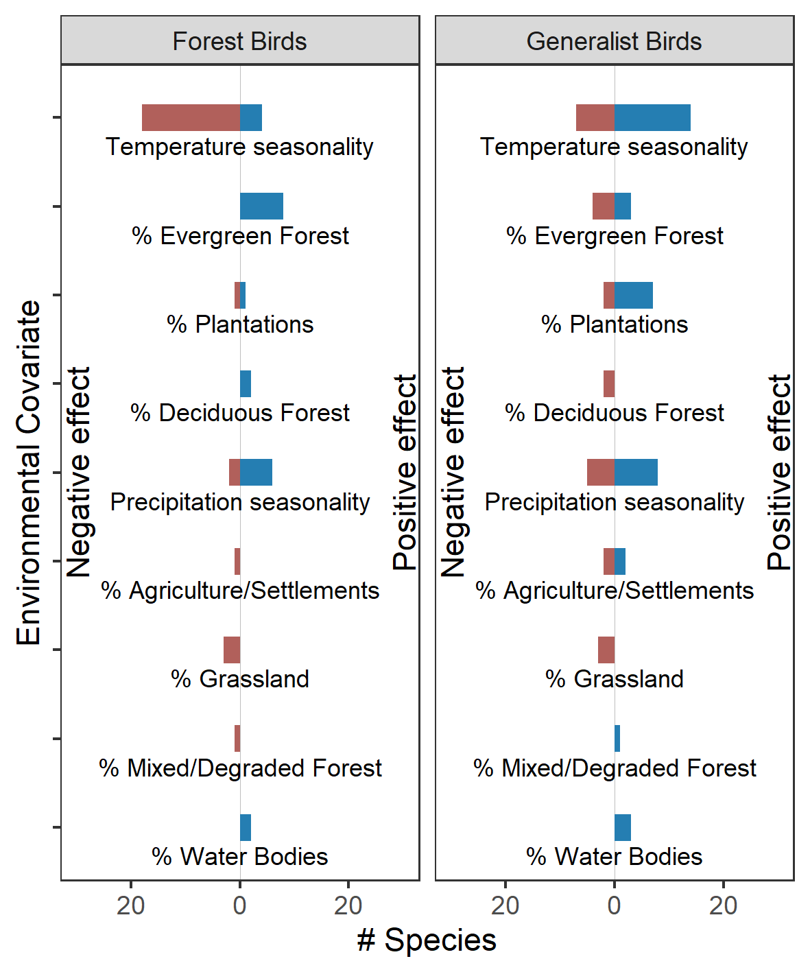
Environmental predictors and species-specific associations The direction of association between species-specific probability of occupancy and climatic and landscape predictors is shown here (as a function of habitat preference). Blue colors show the number of species that are positively associated with a climatic/landscape predictor while red colors show the number of species that are negatively associated with a climatic/landscape predictor (see Table 1 for the number of forest/generalist species that show positive/negative association with each of the predictors).

References

Bartoń, Kamil. 2020. MuMIn: Multi-Model Inference. Manual.

Burnham, Kenneth P., and David R. Anderson. 2002. Model Selection and Multimodel Inference: A Practical Information-Theoretic Approach. Second. New York: Springer-Verlag. https://doi.org/10.1007/b97636.

Burnham, Kenneth P., David R. Anderson, and Kathryn P. Huyvaert. 2011. “AIC Model Selection and Multimodel Inference in Behavioral Ecology: Some Background, Observations, and Comparisons.” Behavioral Ecology and Sociobiology 65 (1): 23–35. https://doi.org/10.1007/s00265-010-1029-6.

Elsen, Paul R., Morgan W. Tingley, Ramnarayan Kalyanaraman, Krishnamurthy Ramesh, and David S. Wilcove. 2017. “The Role of Competition, Ecotones, and Temperature in the Elevational Distribution of Himalayan Birds.” Ecology 98 (2): 337–48. https://doi.org/10.1002/ecy.1669.