Section 2 Selecting species of interest
Prior to preparing eBird data for occupancy modeling, we selected a list of species using a simple and objective criteria. Our primary focus is to understand how terrestrial bird species occupancy (largely passerine species) varied as a function of climate and land cover across the Nilgiri and the Anamalai hills of the Western Ghats.
We derived this list from inclusion criteria adapted from the State of India’s Birds 2020 (Viswanathan et al. 2020). Initially, we considered all species reported on eBird that occurred within the outlines of our study area. We then added a filter to consider only terrestrial birds and removed species that are often easily confused for their congeners (eg. green/greenish warbler). In addition, we considered only those species that had a minimum of 1000 detections each between 2013 and 2021. Next, the study area was divided into 25 x 25 km cells following Viswanathan et al. (2020). We then kept only those species that occurred in at least 5% of all checklists across half of the 25 x 25 km cells from where they have been reported (there are 42 unique 25 x 25 km grid cells across our study area). We used the above criteria to ensure as much uniform sampling of a species as possible across our study area and to reduce any erroneous associations between environmental drivers and species occupancy. This resulted in a total of 79 species, prior to occupancy modeling.
This script shows the proportion of checklists that report a particular species across every 25km by 25km grid across the Nilgiris and the Anamalais. Using this analysis, we arrived at a final list of species for occupancy modeling.
2.1 Prepare libraries
# load libraries
library(data.table)
library(readxl)
library(magrittr)
library(stringr)
library(dplyr)
library(tidyr)
library(readr)
library(ggplot2)
library(ggthemes)
library(scico)
# round any function
round_any <- function(x, accuracy = 25000) {
  round(x / accuracy) * accuracy
}

# set file paths for auk functions
# To use these two datasets, please download the latest versions from https://ebird.org/data/download and set the file path accordingly. Since these two datasets are extremely large, we have not uploaded the same to github.
# In this study, the version of data loaded corresponds to November 2021.

f_in_ebd <- file.path("data/ebd_IN_relNov-2021.txt")
f_in_sampling <- file.path("data/ebd_sampling_relNov-2021.txt")
2.2 Subset species by geographical confines of the study area
# read in shapefile of the study area to subset by bounding box
library(sf)
wg <- st_read("data/spatial/hillsShapefile/Nil_Ana_Pal.shp")
box <- st_bbox(wg)
# read in data and subset
# To access the latest dataset, please visit: https://ebird.org/data/download and set the file path accordingly.
ebd <- fread("data/ebd_IN_relNov-2021.txt")
ebd <- ebd[between(LONGITUDE, box["xmin"], box["xmax"]) &
  between(LATITUDE, box["ymin"], box["ymax"]), ]
ebd <- ebd[year(`OBSERVATION DATE`) >= 2013, ]
# make new column names
newNames <- str_replace_all(colnames(ebd), " ", "_") %>%
  str_to_lower()
setnames(ebd, newNames)
# keep useful columns
columnsOfInterest <- c(
  "common_name", "scientific_name", "observation_count", "locality",
  "locality_id", "locality_type", "latitude",
  "longitude", "observation_date", "sampling_event_identifier"
)
ebd <- ebd[, ..columnsOfInterest]
2.3 Subset an initial list of terrestrial birds based on a) minimum of 1000 detections between 2013-2021 and b) remove species that are often easily confused with congeners
# Convert all presences marked 'X' as '1'
ebd <- ebd %>%
  mutate(observation_count = ifelse(observation_count == "X",
    "1", observation_count
  ))

# Convert observation count to numeric
ebd$observation_count <- as.numeric(ebd$observation_count)

totCount <- ebd %>%
  dplyr::select(scientific_name, common_name, observation_count) %>%
  group_by(scientific_name, common_name) %>%
  summarise(tot = sum(observation_count))

# subset species with a min of 1000 detections
tot1000 <- totCount %>%
  filter(tot > 1000)

species1000 <- tot1000$scientific_name

ebd1000 <- ebd[scientific_name %in% species1000, ]

# Beginning with 3.37 million observations of 684 species in eBird that occurred within the outlines of our study area (Fig. 1), over the years 2013–2021, we retained only those species that had a minimum of 1,000 detections each between 2013 and 2021 (347 species remaining; 3.33 million observations). Next, we divided the study area into 25x25 km cells following State of India’s Birds 2020 methodology. We kept only those species that occurred in at least 5% of all checklists across half of the grids (42 unique grid cells) from which they had been reported.

# export the above list as .csv to carry out initial filtering based on natural history
write.csv(totCount, "data/species_list.csv", row.names = F)
2.4 Read subset of species following filtering and removal of waterbirds, raptors, and other noctural species
2.5 Load raw data for locations
Add a spatial filter and assign grids of 25km x 25km.
# strict spatial filter and assign grid
locs <- ebd[, .(longitude, latitude)]
# transform to UTM and get 25km boxes
coords <- setDF(locs) %>%
  st_as_sf(coords = c("longitude", "latitude")) %>%
  `st_crs<-`(4326) %>%
  bind_cols(as.data.table(st_coordinates(.))) %>%
  st_transform(32643) %>%
  mutate(id = 1:nrow(.))
# convert wg to UTM for filter
wg <- st_transform(wg, 32643)
coords <- coords %>%
  filter(id %in% unlist(st_contains(wg, coords))) %>%
  rename(longitude = X, latitude = Y) %>%
  bind_cols(as.data.table(st_coordinates(.))) %>%
  st_drop_geometry() %>%
  as.data.table()
# remove unneeded objects
rm(locs)
gc()
coords <- coords[, .N, by = .(longitude, latitude, X, Y)]
ebd <- merge(ebd, coords, all = FALSE, by = c("longitude", "latitude"))
ebd <- ebd[(longitude %in% coords$longitude) &
  (latitude %in% coords$latitude), ]
2.6 Get proportional obs counts in 25km cells
# round to 25km cell in UTM coords
ebd[, `:=`(X = round_any(X), Y = round_any(Y))]
# count checklists in cell
ebd_summary <- ebd[, nchk := length(unique(sampling_event_identifier)),
  by = .(X, Y)
]
# count checklists reporting each species in cell and get proportion
ebd_summary <- ebd_summary[, .(nrep = length(unique(
  sampling_event_identifier
))),
by = .(X, Y, nchk, scientific_name)
]
ebd_summary[, p_rep := nrep / nchk]
# filter for soi
ebd_summary <- ebd_summary[scientific_name %in% speciesOfInterest, ]
# complete the dataframe for no reports
# keep no reports as NA --- allows filtering based on proportion reporting
ebd_summary <- setDF(ebd_summary) %>%
  complete(
    nesting(X, Y), scientific_name # ,
    # fill = list(p_rep = 0)
  ) %>%
  filter(!is.na(p_rep))
2.7 Which species are reported sufficiently in checklists?
# A total of 42 unique grids (of 25km by 25km) across the study area
# total number of checklists across unique grids
tot_n_chklist <- ebd_summary %>%
  distinct(X, Y, nchk)
# species-specific number of grids
spp_grids <- ebd_summary %>%
  group_by(scientific_name) %>%
  distinct(X, Y) %>%
  count(scientific_name,
    name = "n_grids"
  )
# Write the above two results
write_csv(tot_n_chklist, "data/01_nchk_per_grid.csv")
write_csv(spp_grids, "data/01_ngrids_per_spp.csv")

# left-join the datasets
ebd_summary <- left_join(ebd_summary, spp_grids, by = "scientific_name")
# check the proportion of grids across which this cut-off is met for each species
# Is it > 90% or 70%?
# For example, with a 3% cut-off, ~100 species are occurring in >50%
# of the grids they have been reported in
p_cutoff <- 0.05 # Proportion of checklists a species has been reported in
grid_proportions <- ebd_summary %>%
  group_by(scientific_name) %>%
  tally(p_rep >= p_cutoff) %>%
  mutate(prop_grids_cut = n / (spp_grids$n_grids)) %>%
  arrange(desc(prop_grids_cut))
grid_prop_cut <- filter(
  grid_proportions,
  prop_grids_cut >= p_cutoff
)
# Write the results
write_csv(grid_prop_cut, "data/01_chk_5_percent.csv")

# Identifying the number of species that occur in potentially <5% of all lists
total_number_lists <- sum(tot_n_chklist$nchk)
spp_sum_chk <- ebd_summary %>%
  distinct(X, Y, scientific_name, nrep) %>%
  group_by(scientific_name) %>%
  mutate(sum_chk = sum(nrep)) %>%
  distinct(scientific_name, sum_chk)
# Approximately 90 to 100 species occur in >5% of all checklists
prop_all_lists <- spp_sum_chk %>%
  mutate(prop_lists = sum_chk / total_number_lists) %>%
  arrange(desc(prop_lists))
2.8 Figure: Checklist distribution
# add land
library(rnaturalearth)
land <- ne_countries(
  scale = 50, type = "countries", continent = "asia",
  country = "india",
  returnclass = c("sf")
)
# crop land
land <- st_transform(land, 32643)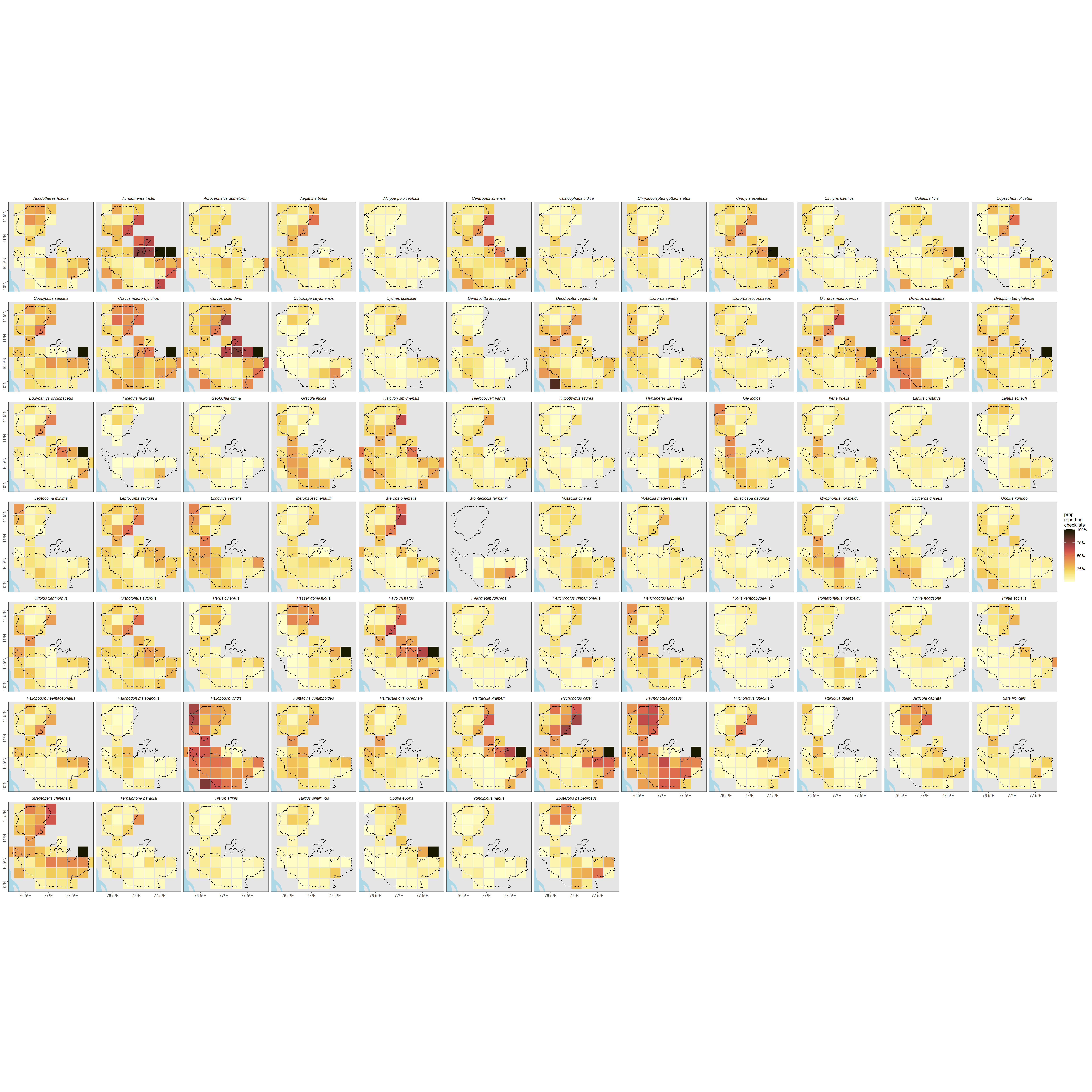
Proportion of checklists reporting a species in each grid cell (25km side) between 2013 and 2021. Checklists were filtered to be within the boundaries of the Nilgiris and the Anamalai hills (black outline), but rounding to 25km cells may place cells outside the boundary. Deeper shades of red indicate a higher proportion of checklists reporting a species.
2.9 Prepare the species list
References
Viswanathan, A., A. Reddy, A. Deomurari, K. Suryawanshi, M. D. Madhusudan, M. Kaushik, P. J, R. Jayapal, and S. & Quader. 2020. State of India’s Birds 2020: Background and Methodology. Manual.