Section 4 Preparing Environmental Predictors
In this script, we processed climatic and landscape predictors for occupancy modeling.
All climatic data was obtained from https://chelsa-climate.org/bioclim/ All landscape data was derived from a high resolution land cover map (Roy et al. 2015). This map provides sufficient classes to achieve a high land cover resolution and can be accessed here (https://daac.ornl.gov/VEGETATION/guides/Decadal_LULC_India.html)
The goal here is to resample all rasters so that they have the same resolution of 1km cells.
4.1 Prepare libraries
We load some common libraries for raster processing and define a custom mode function.
# load libs
library(raster)
library(stringi)
library(glue)
library(gdalUtils)
library(purrr)
library(dplyr)
library(tidyr)
library(tibble)

# for plotting
library(viridis)
library(colorspace)
library(tmap)
library(scales)
library(ggplot2)
library(patchwork)

# prep mode function to aggregate
funcMode <- function(x, na.rm = T) {
  ux <- unique(x)
  ux[which.max(tabulate(match(x, ux)))]
}

# a basic test
assertthat::assert_that(funcMode(c(2, 2, 2, 2, 3, 3, 3, 4)) == as.character(2),
  msg = "problem in the mode function"
) # works

# get ci func
ci <- function(x) {
  qnorm(0.975) * sd(x, na.rm = T) / sqrt(length(x))
}
4.2 Prepare spatial extent
We prepare a 30km buffer around the boundary of the study area. This buffer will be used to mask the landscape rasters.The buffer procedure is done on data transformed to the UTM 43N CRS to avoid distortions.
4.3 Prepare terrain rasters
We prepare the elevation data which is an SRTM raster layer, and derive the slope and aspect from it after cropping it to the extent of the study site buffer. Please download the latest version of the SRTM raster layer from https://www.worldclim.org/data/worldclim21.html
# load elevation and crop to hills size, then mask by study area
alt <- raster("data/spatial/Elevation/alt") # this layer is not added to github as a result of its large size and can be downloaded from the above link
alt.hills <- raster::crop(alt, as(buffer, "Spatial"))
rm(alt)
gc()

# get slope and aspect
slopeData <- raster::terrain(x = alt.hills, opt = c("slope", "aspect"))
elevData <- raster::stack(alt.hills, slopeData)
rm(alt.hills)
gc()
4.4 Prepare CHELSA rasters
CHELSA rasters can be downloaded using the get_chelsa.sh shell script, which is a wget command pointing to the envidatS3.txt file.
4.4.1 Prepare BIOCLIM 4a and 15
We prepare the CHELSA rasters for seasonality in temperature (Bio 4a) and seasonality in precipitation (Bio 15) in the same way, reading them in, cropping them to the study site buffer extent, and handling the temperature layer values which we divide by 10. The CHELSA rasters can be downloaded from https://chelsa-climate.org/bioclim/
# list chelsa files
# the chelsa data can be downloaded from the aforementioned link. They haven't been uploaded to github as a result of its large size.
chelsaFiles <- list.files("data/chelsa/",
  full.names = TRUE,
  recursive = TRUE,
  pattern = "bio10"
)

# gather chelsa rasters
chelsaData <- purrr::map(chelsaFiles, function(chr) {
  a <- raster(chr)
  crs(a) <- crs(elevData)
  a <- crop(a, as(buffer, "Spatial"))
  return(a)
})

# divide temperature by 10
chelsaData[[1]] <- chelsaData[[1]] / 10

# stack chelsa data
chelsaData <- raster::stack(chelsaData)
4.4.2 Prepare BIOCLIM 4a
if (file.exists("data/chelsa/CHELSA_bio10_4a.tif")) {
  message("Bio 4a already exists, will be overwritten")
}
Bioclim 4a, the coefficient of variation temperature seasonality is calculated as
\[Bio\ 4a = \frac{SD\{ Tkavg_1, \ldots Tkavg_{12} \}}{(Bio\ 1 + 273.15)} \times 100\]
where \(Tkavg_i = (Tkmin_i + Tkmax_i) / 2\)
Here, we use only the months of December and Jan – May for winter temperature variation.
# list rasters by pattern
patterns <- c("tmin", "tmax")

# list the filepaths
tkAvg <- map(patterns, function(pattern) {
  # list the paths
  files <- list.files(
    path = "data/chelsa",
    full.names = TRUE,
    recursive = TRUE,
    pattern = pattern
  )
})

# print crs elev data for sanity check --- basic WGS84
crs(elevData)

# now run over the paths and read as rasters and crop by buffer
tkAvg <- map(tkAvg, function(paths) {
  # going over the file paths, read them in as rasters, convert CRS and crop
  tempData <- map(paths, function(path) {
    # read in
    a <- raster(path)
    # assign crs
    crs(a) <- crs(elevData)
    # crop by buffer, will throw error if CRS doesn't match
    a <- crop(a, as(buffer, "Spatial"))
    # return a
    a
  })
  # convert each to kelvin, first dividing by 10 to get celsius
  tempData <- map(tempData, function(tmpRaster) {
    tmpRaster <- (tmpRaster / 10) + 273.15
  })
})

# assign names
names(tkAvg) <- patterns

# go over the tmin and tmax and get the average monthly temp
tkAvg <- map2(tkAvg[["tmin"]], tkAvg[["tmax"]], function(tmin, tmax) {
  # return the mean of the corresponding tmin and tmax
  # still in kelvin
  calc(stack(tmin, tmax), fun = mean)
})

# calculate Bio 4a
bio_4a <- (calc(stack(tkAvg), fun = sd) / (chelsaData[[1]] + 273.15)) * 100
names(bio_4a) <- "CHELSA_bio10_4a"
# save bio_4a
writeRaster(bio_4a, filename = "data/chelsa/CHELSA_bio10_4a.tif", overwrite = T)
4.4.3 Prepare Bioclim 15
if (file.exists("data/chelsa/CHELSA_bio10_15.tif")) {
  message("Bio 15 already exists, will be overwritten")
}
Bioclim 15, the coefficient of variation precipitation (in our area, rainfall) seasonality is calculated as
\[Bio\ 15 = \frac{SD\{ PPT_1, \ldots PPT_{12} \}}{1 + (Bio\ 12 / 12)} \times 100\]
where \(PPT_i\) is the monthly precipitation.
Here, we use only the months of December and Jan – May for winter rainfall variation.
# list rasters by pattern
pattern <- "prec"

# list the filepaths
pptTotal <- list.files(
  path = "data/chelsa",
  full.names = TRUE,
  recursive = TRUE,
  pattern = pattern
)

# print crs elev data for sanity check --- basic WGS84
crs(elevData)

# now run over the paths and read as rasters and crop by buffer
pptTotal <- map(pptTotal, function(path) {
  a <- raster(path)
  # assign crs
  crs(a) <- crs(elevData)
  # crop by buffer, will throw error if CRS doesn't match
  a <- crop(a, as(buffer, "Spatial"))
  # return a
  a
})

# calculate Bio 4a
bio_15 <- (calc(stack(pptTotal), fun = sd) / (1 + (chelsaData[[2]] / 12))) * 100
names(bio_15) <- "CHELSA_bio10_15"
# save bio_4a
writeRaster(bio_15, filename = "data/chelsa/CHELSA_bio10_15.tif", overwrite = T)
4.4.4 Stack terrain and climate
We stack the terrain and climatic rasters.
4.5 Resample landcover from 10m to 1km
We read in a land cover classified image and resample that using the mode function to a 1km resolution. Please note that the resampling process need not be carried out as it has been done already and the resampled raster can be loaded with the subsequent code chunk.
# read in landcover raster location
# To access the land cover data, please visit: https://daac.ornl.gov/VEGETATION/guides/Decadal_LULC_India.html

landcover <- "data/landUseClassification/landcover_roy_2015/"

# read in and crop
landcover <- raster(landcover)
buffer_utm <- st_transform(buffer, 32643)
landcover <- crop(
  landcover,
  as(
    buffer_utm,
    "Spatial"
  )
)

# read reclassification matrix
reclassification_matrix <- read.csv("data/landUseClassification/LandCover_ReclassifyMatrix_2015.csv")
reclassification_matrix <- as.matrix(reclassification_matrix[, c("V1", "To")])

# reclassify
landcover_reclassified <- reclassify(
  x = landcover,
  rcl = reclassification_matrix
)

# write to file
writeRaster(landcover_reclassified,
  filename = "data/landUseClassification/landcover_roy_2015_reclassified.tif",
  overwrite = TRUE
)

# check reclassification
plot(landcover_reclassified)

# get extent
e <- bbox(raster(landcover))

# init resolution
res_init <- res(raster(landcover))

# res to transform to 1000m
res_final <- res_init * (1000 / res_init)

# use gdalutils gdalwarp for resampling transform
# to 1km from 10m
gdalUtils::gdalwarp(
  srcfile = "data/landUseClassification/landcover_roy_2015_reclassified.tif",
  dstfile = "data/landUseClassification/lc_01000m.tif",
  tr = c(res_final), r = "mode", te = c(e)
)
We compare the frequency of landcover classes between the original raster and the resampled 1km raster to be certain that the resampling has not resulted in drastic misrepresentation of the frequency of any landcover type. This comparison is made using the figure below.
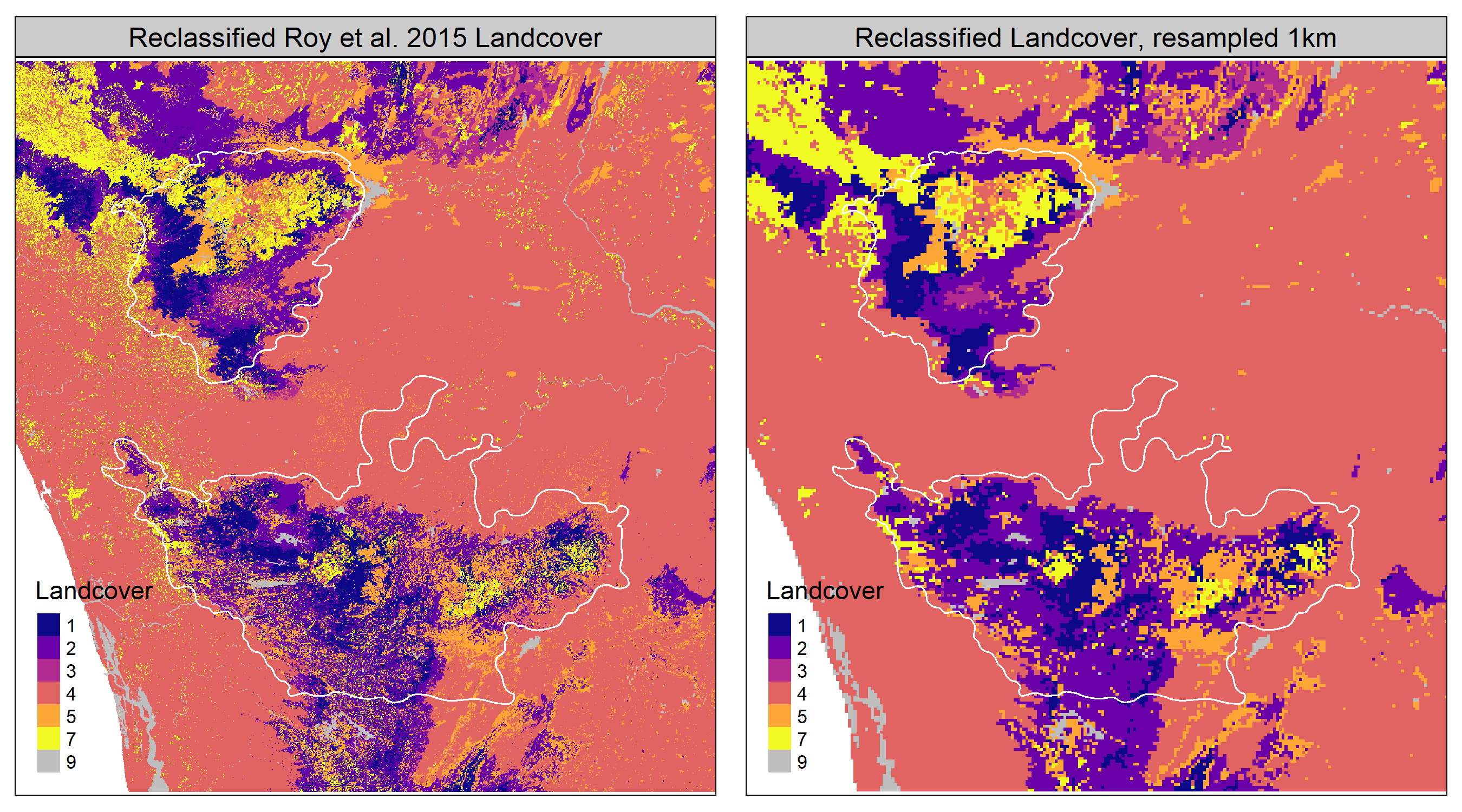
Resampling the Roy et al. (2015) landcover raster, reclassified into 7 main classes, to a resolution of 1km, preserves the important features of landcover over the study area.
4.6 Resample other rasters to 1km
We now resample all other rasters to a resolution of 1km.
4.6.1 Read in resampled landcover
Here, we read in the 1km landcover raster and set 0 to NA.
4.6.2 Reproject environmental data using landcover as a template
# resample to the corresponding landcover data
env_data_resamp <- projectRaster(
  from = env_data, to = lc_data,
  crs = crs(lc_data), res = res(lc_data)
)

# export as raster stack
land_stack <- stack(env_data_resamp, lc_data)

# get names
land_names <- glue('data/spatial/landscape_resamp{c("01")}_km.tif')

# write to file
raster::writeRaster(
  land_stack, filename = as.character(land_names),
  overwrite = TRUE
)
4.7 Climate variables in relation to elevation
4.7.1 Load resampled environmental rasters
# read landscape prepare for plotting
landscape <- stack("data/spatial/landscape_resamp01_km.tif")

# get proper names
elev_names <- c("elev", "slope", "aspect")
chelsa_names <- c("bio_4a", "bio_15")

names(landscape) <- glue('{c(elev_names, chelsa_names, "landcover")}')
# make duplicate stack
land_data <- landscape[[c("elev", chelsa_names)]]
# convert to list
land_data <- as.list(land_data)
# map get values over the stack
land_data <- purrr::map(land_data, getValues)
names(land_data) <- c("elev", chelsa_names)
# conver to dataframe and round to 200m
land_data <- bind_cols(land_data)
land_data <- drop_na(land_data) %>%
mutate(elev_round = plyr::round_any(elev, 200)) %>%
dplyr::select(-elev) %>%
pivot_longer(
cols = contains("bio"),
names_to = "clim_var"
) %>%
group_by(elev_round, clim_var) %>%
summarise_all(.funs = list(~ mean(.), ~ ci(.)))Figure code is hidden in versions rendered as HTML or PDF.
4.8 Climate across land cover types
Get climate values per (re-classified) landcover type from the 1km resampled raster.
# make duplicate stack again
lc_clim_data <- landscape[[c("landcover", chelsa_names)]]

# convert to list
lc_clim_data <- as.list(lc_clim_data)

# map get values over the stack
lc_clim_data <- purrr::map(lc_clim_data, getValues)
names(lc_clim_data) <- c("landcover", chelsa_names)

# conver to dataframe for histogram
lc_clim_data <- bind_cols(lc_clim_data)

# pivot long
lc_clim_data <- pivot_longer(
  lc_clim_data,
  cols = contains("bio"),
  names_to = "climvar"
)

# make landcover factor
lc_clim_data <- mutate(
  lc_clim_data,
  landcover = factor(landcover)
)

# filter bio
lc_clim_data <- filter(
  lc_clim_data,
  !is.na(landcover)
)

# split by variable
lc_clim_data <- nest(lc_clim_data, data = c("landcover", "value"))

# assign names
lc_clim_data$climvar_name <- c(
  "Temperature seasonality",
  "Precipitation seasonality"
)
Plot density plots of climate seasonality per LC type.
# make labels
lc_labels <- c(
  "Evergreen", "Deciduous",
  "Mixed./Degr.", "Agri./Settl.",
  "Grassland", "Plantation",
  "Waterbody"
)
names(lc_labels) <- c(seq(5), 7, 9)

# plots
lc_clim_plots <- pmap(
  lc_clim_data,
  function(climvar_name, data, climvar) {
    p <- data %>%
      ggplot() +
      geom_histogram(
        aes(
          x = value, y = ..density..,
          fill = ..x..
        ),
        show.legend = F
      ) +
      theme_test(base_family = "Arial") +
      theme(
        legend.key.width = unit(2, units = "mm"),
        axis.text.y = element_blank(),
        axis.text.x = element_text(size = 6, angle = 45),
        axis.ticks.y = element_blank(),
        strip.background = element_blank(),
        strip.text = element_text(size = 6, face = "bold")
      ) +
      facet_grid(
        ~landcover,
        labeller = labeller(
          landcover = lc_labels
        )
      ) +
      labs(
        x = glue("{climvar_name}"),
        y = "Density"
      )
    if (climvar == "bio_1") {
      p <- p +
        scale_fill_continuous_diverging(
          palette = "Blue-Red 2",
          mid = 29.5
        )
    } else {
      p <- p +
        scale_x_continuous(
          limits = c(200, 500)
        ) +
        scale_fill_continuous_diverging(
          palette = "Blue-Yellow 2",
          mid = 350
        )
    }

    p
  }
)

# save to file and add figure
fig_lc_clim <-
  wrap_plots(lc_clim_plots, ncol = 1) &
    plot_annotation(tag_levels = "A")

# save as png
ggsave(fig_lc_clim,
  filename = "figs/fig_lc_climate.png",
  height = 4, width = 6.5, device = png(), dpi = 300
)
4.9 Land cover type in relation to elevation
# get data from landscape rasters
lc_elev <- tibble(
  elev = getValues(landscape[["elev"]]),
  landcover = getValues(landscape[["landcover"]])
)

# process data for proportions
lc_elev <- lc_elev %>%
  filter(!is.na(landcover), !is.na(elev)) %>%
  # round elev to 100m
  mutate(elev = plyr::round_any(elev, 100)) %>%
  count(elev, landcover) %>%
  group_by(elev) %>%
  mutate(prop = n / sum(n))

# fill out lc elev
lc_elev_canon <- crossing(
  elev = unique(lc_elev$elev),
  landcover = unique(lc_elev$landcover)
)

# bind with lcelev
lc_elev <- full_join(lc_elev, lc_elev_canon)

# convert NA to zero
lc_elev <- replace_na(lc_elev, replace = list(n = 0, prop = 0))
Figure code is hidden in versions rendered as HTML and PDF.
4.10 Main Text Figure 2
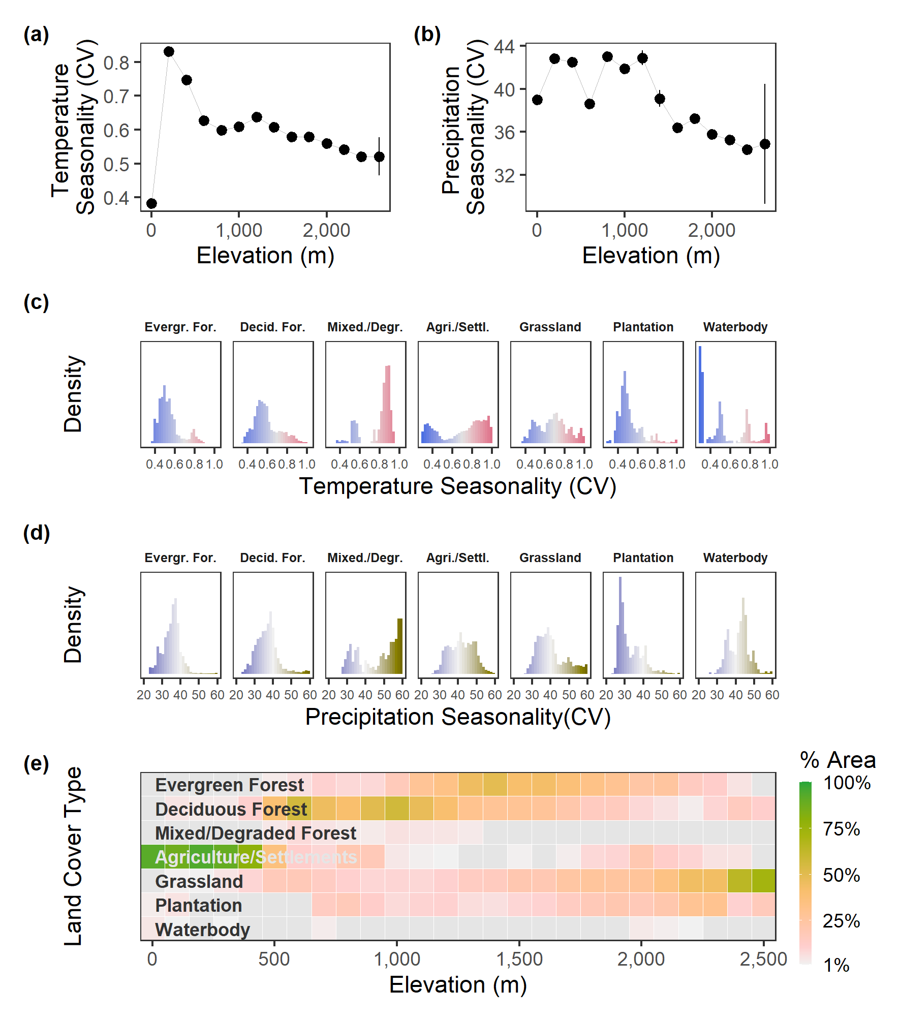
Climate and land cover vary strongly along the elevation gradient in the Nilgiri and Anamalai Hills. Both (a) temperature seasonality and (b) precipitation seasonality, between the months of December and May, declines with increasing elevation across the Nilgiri and Anamalai Hills. Climatic variation is not very strongly associated with land cover type, as both natural habitats such as forests, and human-associated habitat types such as plantations show low seasonality in (c) temperature, and (d) precipitation. (e) Most elevations host a range of land cover types: while human-associated habitats such as agriculture are concentrated at lower elevations, and more natural types such as grasslands and forests are associated with higher elevations, each of these types is also found outside their characteristic elevational bands. We calculated climate seasonalities (BIOCLIM 4a and 15: temperature and precipitation, respectively) using CHELSA data over 1979 – 2013, from December to May (Karger et al. 2017), and present mean seasonality values (vertical bars show standard deviation) for every 200 m elevational band. Land cover types were taken from a reclassification of Roy et al. (2015; see main text) at 100 m elevational bands. Land cover types covering < 1% of an elevational band are shaded grey. All landscape layers were first resampled to 1 km resolution.