Section 6 Examining Spatial Sampling Bias

The goal of this section is to show how far each checklist location is from the nearest road, and how far each site is from its nearest neighbour. This follows finding the pairwise distance between a large number of unique checklist locations to a vast number of roads, as well as to each other.

6.1 Prepare libraries

# load libraries
# for data
library(sf)
library(rnaturalearth)
library(dplyr)
library(readr)
library(purrr)

# for plotting
library(scales)
library(ggplot2)
library(ggspatial)
library(colorspace)

# round any function
round_any <- function(x, accuracy = 20000) {
  round(x / accuracy) * accuracy
}
# ci function
ci <- function(x) {
  qnorm(0.975) * sd(x, na.rm = TRUE) / sqrt(length(x))
}

6.2 Read checklist data

Read in checklist data with distance to nearest neighbouring site, and the distance to the nearest road.

# read from local file
chkCovars <- read_csv("data/03_data-covars-perChklist.csv")

6.2.1 Spatially explicit filter on checklists

We filter the checklists by the boundary of the study area. This is not the extent.

chkCovars <- st_as_sf(chkCovars, coords = c("longitude", "latitude")) %>%
  `st_crs<-`(4326) %>%
  st_transform(32643)

# read wg
wg <- st_read("data/spatial/hillsShapefile/Nil_Ana_Pal.shp") %>%
  st_transform(32643)
# get bounding box
bbox <- st_bbox(wg)

# spatial subset
chkCovars <- chkCovars %>%
  mutate(id = 1:nrow(.)) %>%
  filter(id %in% unlist(st_contains(wg, chkCovars)))

6.2.2 Get background land for plotting

# add land
land <- ne_countries(
  scale = 50, type = "countries", continent = "asia",
  country = "india",
  returnclass = c("sf")
) %>%
  st_transform(32643)

# add roads data
roads <- st_read("data/spatial/roads_studysite_2019/roads_studysite_2019.shp") %>%
  st_transform(32643)

6.3 Prepare Main Text Figure 3

6.3.1 Prepare histogram of distance to roads

Figure code is hidden in versions rendered as HTML or PDF.

6.3.2 Table: Distance to roads

# write the mean and ci95 to file
chkCovars %>%
  st_drop_geometry() %>%
  dplyr::select(dist_road, nnb) %>%
  tidyr::pivot_longer(
    cols = c("dist_road", "nnb"),
    names_to = "variable"
  ) %>%
  group_by(variable) %>%
  summarise_at(
    vars(value),
    list(~ mean(.), ~ sd(.), ~ min(.), ~ max(.))
  ) %>%
  write_csv("data/results/distance_roads_sites.csv")

6.3.3 Distance to nearest neighbouring site

# get unique locations from checklists
locs_unique <- cbind(
  st_drop_geometry(chkCovars),
  st_coordinates(chkCovars)
) %>%
  as_tibble()

locs_unique <- distinct(locs_unique, X, Y, .keep_all = T)

Figure code is hidden in versions rendered as HTML and PDF.

6.3.4 Spatial distribution of distances to neighbours

Figure code is hidden in HTML and PDF versions, consult the Rmarkdown file.

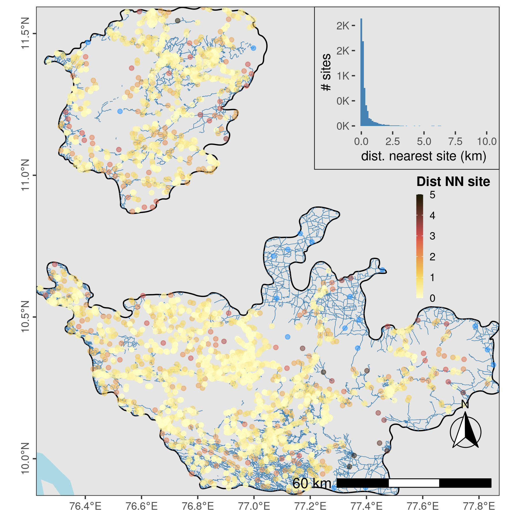
Most observation sites are within 300m of another site.

6.4 Figure: Spatial sampling bias

# get locations
points <- chkCovars %>%
  bind_cols(as_tibble(st_coordinates(.))) %>%
  st_drop_geometry() %>%
  mutate(X = round_any(X, 2500), Y = round_any(Y, 2500))

# count points
points <- count(points, X, Y)

Figure code is hidden in versions rendered as HTML and PDF.

# save as png
ggsave(
  fig_checklists_grid,
  filename = "figs/fig_spatial_bias.png"
)

# save figure as Robject for next plot
save(fig_checklists_grid, file = "data/fig_checklists_grid.Rds")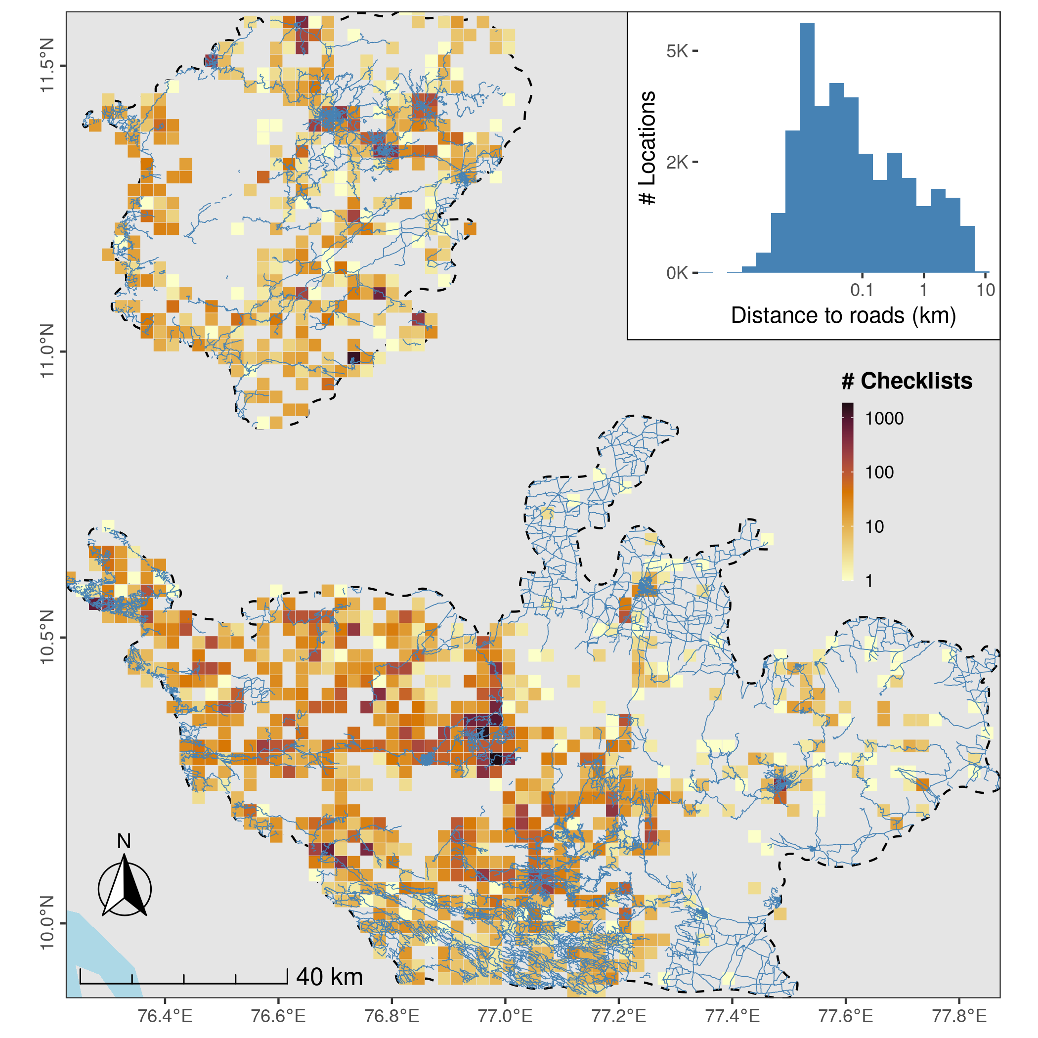

Sampling effort across the Nilgiri and Anamalai Hills, in the form of eBird checklists reported by birdwatchers, mostly takes place along roads, with the majority of checklists located < 1 km from a roadway (see distribution in inset), and therefore, only about 300m, on average, from the location of another checklist. Each cell here is 2.5km x 2.5km.