Section 11 Predicting species-specific occupancy as a function of significant predictors

This script plots species-specific probabilities of occupancy as a function of significant environmental predictors and maps occupancy across the study area for a given list of species and significant predictors.

11.1 Prepare libraries

# to handle data
library(dplyr)
library(readr)
library(tidyr)
library(purrr)
library(stringr)
library(glue)
# library(data.table)

# plotting
library(ggplot2)
library(patchwork)

11.2 Read data

# read coefficient effect data
data <- read_csv("data/results/data_predictor_effect.csv")

# check for a predictor column
assertthat::assert_that(
  all(c("predictor", "coefficient", "se") %in% colnames(data)),
  msg = "make_response_data: data must have columns called 'predictor',
    'coefficient', and 'se'"
)

11.3 Prepare predictor data

# preparep predictors - now look only for any digits
predictors <- c("bio\\d+", glue("lc_0{seq(9)}"))

# prepare predictor search strings and scaling power
preds <- glue("({predictors})")
preds <- str_flatten(preds, collapse = "|")

# some way of identifying square terms
power <- (str_extract(data$predictor, "Ibio"))
power[!is.na(power)] = 2
power[is.na(power)] <- 1
power = as.numeric(power)

# assign predictor name and power
data <-
  mutate(
  data,
  predictor = str_extract(predictor, preds),
  power = power
)

11.4 Get predictor responses

# make predictor sequences
data <- mutate(
  data,
  pred_val = map(
    predictor,
    function(x) {
      seq(0, 1, 0.05)
    }
  ),
  #handle squared terms
  pred_val_pow = purrr::map2(
    pred_val, power,
    function(x, y) {
      x^y
    }
))


# get coefficient and error times terms
data_resp <- mutate(
  data,
  response = map2(
    pred_val_pow, coefficient,
    function(x, y) {
      x * y
    }
  ),
  resp_var = map2(
    pred_val_pow, se,
    function(x, y) {
      x * y
    }
  )
)

11.5 Get probability of occupancy

# unnest and get responses
data_resp <- unnest(
  data_resp,
  cols = c("response", "resp_var", "pred_val")
)

# get responses for quadratic terms
data_resp <-
  group_by(
    data_resp,
    scientific_name, predictor, pred_val
  ) %>%
  dplyr::select(-power, -coefficient, -se) %>%
  summarise(
    across(
      .cols = c("response", "resp_var"),
      .fns = sum
    ),
    .groups = "keep"
  )

# get probability of occupancy
data_resp <- ungroup(
  data_resp
) %>%
  mutate(
    p_occu = 1 / (1 + exp(-response)),
    p_occu_low = 1 / (1 + exp(-(response - resp_var))),
    p_occu_high = 1 / (1 + exp(-(response + resp_var)))
  )

11.6 Add scaling for predictors

# scale predictors
scale15 <- c(30, 50) # range of precipitation
scale4 <- c(0, 1) # range of temperatures

# scale bio4a and bio15a by actual values
data_resp <- mutate(
  data_resp,
  pred_val = case_when(
    predictor == "bio4" ~ scales::rescale(pred_val, to = scale4),
    predictor == "bio15" ~ scales::rescale(pred_val, to = scale15),
    T ~ pred_val
  )
)

# make long
data_poccu <- dplyr::select(
  data_resp,
  -response, -resp_var
)

# select species
soi <- c("Irena puella","Leptocoma minima", "Merops leschenaulti","Myophonus horsfieldii")

which_predictors <- c("bio4")

11.6.1 Figure: Occupancy ~ predictors

data_fig <- data_poccu %>%
  filter(
    scientific_name %in% soi,
    predictor %in% which_predictors
  ) %>%
  mutate(
    cat = case_when(
      scientific_name %in% c("Irena puella","Leptocoma minima") ~ "forest",
      T ~ "general"
    )
  )

# split data
data_fig <- nest(
  data_fig,
  -cat
)

# make plots
make_occu_fig <- function(df, this_fill) {
  ggplot(
    df
  ) +
    geom_ribbon(
      aes(
        pred_val,
        ymin = p_occu_low,
        ymax = p_occu_high
      ),
      fill = this_fill,
      alpha = 0.5
    ) +
    geom_line(
      aes(
        pred_val, p_occu
      ),
      size = 1
    ) +
    facet_grid(
      ~scientific_name
    ) +
    theme_test(
      base_family = "Arial"
    ) +
    theme(
      strip.text = element_text(
        face = "italic"
      )
    ) +
    labs(
      x = "Temperature seasonality",
      y = "Probability of occupancy"
    )
}


fig_occu <- map2(data_fig$data, "grey", make_occu_fig)

fig_occu <-
  wrap_plots(
    fig_occu[c(1, 2)],
    ncol = 1, nrow = 2
  ) &
    theme(
      plot.tag = element_text(
        face = "bold"
      )
    )

# save figure
ggsave(
  fig_occu,
  filename = "figs/fig_05.png",
  width = 5, height = 5.5
)

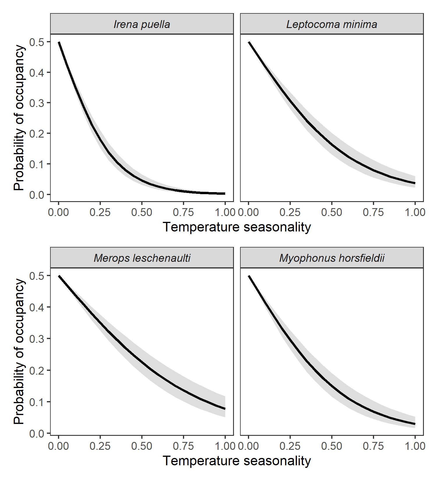
Probability of occupancy as a function of temperature seasonality. Predicted probability of occupancy curves as a function of temperature seasonality for four forest species are shown here. Temperature seasonality is negatively associated with the probability of occupancy of several forest species including the asian fairy-bluebird Irena puella, the crimson-backed sunbird Leptocoma minima, the chestnut-headed bee-eater Merops leschenaulti and the Malabar whistling-thrush Myophonus horsfieldii.

11.6.2 Figures: Occupancy ~ predictors for all species

data_fig <- nest(
  data_poccu,
  -scientific_name, -predictor
)

pred_names <- c(
  "bio4" = "Temp. seasonality",
  "bio15" = "Precip. seasonality",
  "lc_01" = "Evergreen",
  "lc_02" = "Deciduous",
  "lc_03" = "Mixed/degraded",
  "lc_04" = "Agri./Settl.",
  "lc_05" = "Grassland",
  "lc_07" = "Plantation",
  "lc_09" = "Water"
)

pred_names <- tibble(
  name = pred_names,
  predictor = names(pred_names)
)

data_fig <- left_join(
  data_fig,
  pred_names
)

data_fig <- mutate(
  data_fig,
  plots = map(
    data, function(df) {
      ggplot(df) +
        geom_ribbon(
          aes(
            pred_val,
            ymin = p_occu_low,
            ymax = p_occu_high
          ),
          fill = "grey",
          alpha = 0.5
        ) +
        geom_line(
          aes(
            pred_val, p_occu
          )
        ) +
        coord_cartesian(
          ylim = c(0, 1)
        ) +
        theme_test(
          base_family = "Arial"
        ) +
        labs(
          x = "Predictor",
          y = "p(Occupancy)"
        )
    }
  )
)

# add names
data_fig <- mutate(
  data_fig,
  plots = map2(
    plots, name,
    function(p, name) {
      p <- p + labs(
        x = name
      )
    }
  )
)

# summarise as patchwork
data_fig <- group_by(
  data_fig,
  scientific_name
) %>%
  summarise(
    plots = list(
      wrap_plots(
        plots,
        ncol = 5
      )
    )
  )

# add title as sp
data_fig <- mutate(
  data_fig,
  plots = map2(
    plots, scientific_name,
    function(p, name) {
      p <- p & plot_annotation(
        title = name
      )
    }
  )
)

# save images
cairo_pdf(
  filename = "figs/fig_occupancy_predictors.pdf",
  onefile = TRUE, width = 10, height = 2
)
data_fig$plots
dev.off()

11.7 Mapping species occupancy

11.7.1 Read in raster layers

library(terra)
library(sf)

# read saved rasters
lscape = rast("data/spatial/landscape_resamp01_km.tif")

# isolate temperature and rainfall
bio4 = lscape[[4]] 
bio15 = lscape[[5]] # rain

# careful while loading this raster, large size
landcover <- rast("data/landUseClassification/landcover_roy_2015_reclassified.tif")

lc_1km <- rast("data/landUseClassification/lc_01000m.tif")

11.7.2 Split landcover into proportions per 1km

# separate the fine-scale landcover raster into presence-absence of each class
lc_split <- segregate(landcover)

# resample to 1km
# bilinear resampling uses the mean function.
# mean of N 0s and 1s is the proportion of 1s, ie, proportion of each landcover
lc_split <- terra::resample(
  lc_split,
  lc_1km,
  method = "bilinear"
)

# rename rasters
names(lc_split) <- pred_names$name[-c(1, 2)]

# save raster of landcover proportion
terra::writeRaster(
  lc_split,
  filename = "data/spatial/raster_landcover_proportion_1km.tif",
  overwrite=TRUE
)

rm(landcover)
gc()

# plot proportion of landcover classes
png(width = 1200 * 2, height = 1200 * 2, filename = "figs/fig_landcover_proportion_1km.png", res = 300)
plot(
  lc_split,
  col = colorspace::sequential_hcl(20, palette = "Viridis"),
  range = c(0, 1)
)
dev.off()

11.7.3 Prepare climatic layers

# load landcover split
lc_split = terra::rast("data/spatial/raster_landcover_proportion_1km.tif")

11.7.4 Mask by study area

# mask by hills
# run only if required (makes more sense to map to a larger area)
hills = st_read("data/spatial/hillsShapefile/Nil_Ana_Pal.shp") %>% 
  st_transform(32643)

#bio_1 = terra::mask(
#  bio_1,
#  vect(hills)
#)

#bio_12 = terra::mask(
#  bio_12,
#  vect(hills)
#)

# get ranges
range4 <- terra::minmax(bio4)[, 1] 
range15 <- terra::minmax(bio15)[, 1]

# rescale
bio4 <- (bio4 - min(range4)) / (diff(range4))
bio15 <- (bio15 - min(range15)) / (diff(range15))

# project to UTM
climate <- c(bio4, bio15)
names(climate) = c(
  "Temp. seasonality", 
  "Precip. seasonality"
)

climate <- terra::project(
  x = climate, y = lc_1km
)

# make squared terms
climate2 <- climate * climate

# names
names(climate2) = glue("{names(climate)} 2")

# add to landcover proportions and plot
landscape <- c(climate, lc_split)

11.7.5 Plot full bounds of landscape variables

# plot proportion of landcover classes
png(
  width = 1200 * 2, height = 1200 * 2, filename = "figs/fig_landscape_1km.png",
  res = 300
)
plot(
  landscape,
  col = colorspace::sequential_hcl(20, palette = "agSunset", rev = T),
  range = c(0, 1)
)
dev.off()

# add squared terms
landscape <- c(
  climate, climate2, lc_split
)

#landscape = terra::mask(
#  landscape,
#  vect(hills)
#)

11.7.6 Prepare soi predictors

Prepare the soi predictor coefficients as a vector of the same length as the number of raster layers. These will be multiplied with each layer to give the effect of each layer.

# get soi coefs
sp_coefs <- filter(
  data
) %>%
  dplyr::select(
    -pred_val, -pred_val_pow
  )

# add missing landcover classes
sp_preds <- crossing(
  scientific_name = soi,
  predictor = pred_names$predictor,
  power = c(1, 2)
)

# remove squared terms for landcover
sp_preds <- filter(
  sp_preds,
  !(str_detect(predictor, "lc") & power == 2)
)

# correct square LC terms
sp_coefs = mutate(
  sp_coefs,
  power = if_else(
    str_detect(predictor, "lc"),
    1,
    power
  )
)

sp_coefs <- full_join(
  sp_coefs,
  sp_preds
)

# make wide --- this should give no warnings
sp_coefs <-
  pivot_wider(
    sp_coefs,
    id_cols = c("scientific_name"),
    names_from = c("predictor", "power"),
    values_from = "coefficient"
  )

# get into order
sp_coefs <- dplyr::select(
  sp_coefs,
  scientific_name,
  c(
    "bio4_1", "bio15_1",
    "bio4_2", "bio15_2"
  ),
  matches("lc")
)

# get vectors of coefficients
sp_coefs <- nest(
  sp_coefs,
  -scientific_name
)

11.7.7 Prepare species occupancy for SOI

Here, we shall simply multiply each landscape layer with the corresponding predictor coefficient.Where these are not available, we shall simply multiply the corresponding layer with NA. The resulting layers will be summed together to get a single response layer, which will then be inverse logit transformed to get the probability of occupancy.

# multiply coefficients with layers
soi_occu <- map(
  sp_coefs[sp_coefs$scientific_name %in% soi, ]$data,
  .f = function(df) {
    response <- unlist(slice(df, 1), use.names = F) * landscape
    response <- sum(response, na.rm = TRUE) # remove NA layers, i.e., non-sig preds

    # now transform for probability occupancy
    response <- 1 / (1 + exp(-response))
  }
)

# assign names
names(soi_occu) <- soi

# make single stack
soi_occu <- reduce(soi_occu, c)
names(soi_occu) <- c("Irena puella","Leptocoma minima","Merops leschenaulti","Myophonus horsfieldii")

# use stars for plotting with ggplot
library(stars)
library(colorspace)

soi_occu <- st_as_stars(soi_occu)

fig_occu_map <- ggplot() +
  geom_stars(
    data = soi_occu
  ) +
  scale_fill_binned_sequential(
    palette = "Purple-Yellow",
    name = "Probability of Occupancy",
    rev = T,
    limits = c(0, 1),
    breaks = seq(0, 1, 0.1), 
    na.value = "grey99",
    show.limits = T
  ) +
  facet_wrap(
    ~band,
    labeller = labeller(
      band = function(x) str_replace(x, "\\.", " ")
    )
  ) +
  coord_sf(
    crs = 32643,
    expand = FALSE
  ) +
  theme_test() +
  theme(
    # legend.position = "rg",
    axis.title = element_blank(),
    axis.text = element_blank(),
    legend.key.height = unit(10, "mm"),
    legend.key.width = unit(1, "mm"),
    strip.text = element_text(
      face = "italic"
    ),
    legend.title = element_text(
      vjust = 1
    )
  )

# save figure
ggsave(
  fig_occu_map,
  filename = "figs/fig_06.png",
  width = 6, height = 6
)

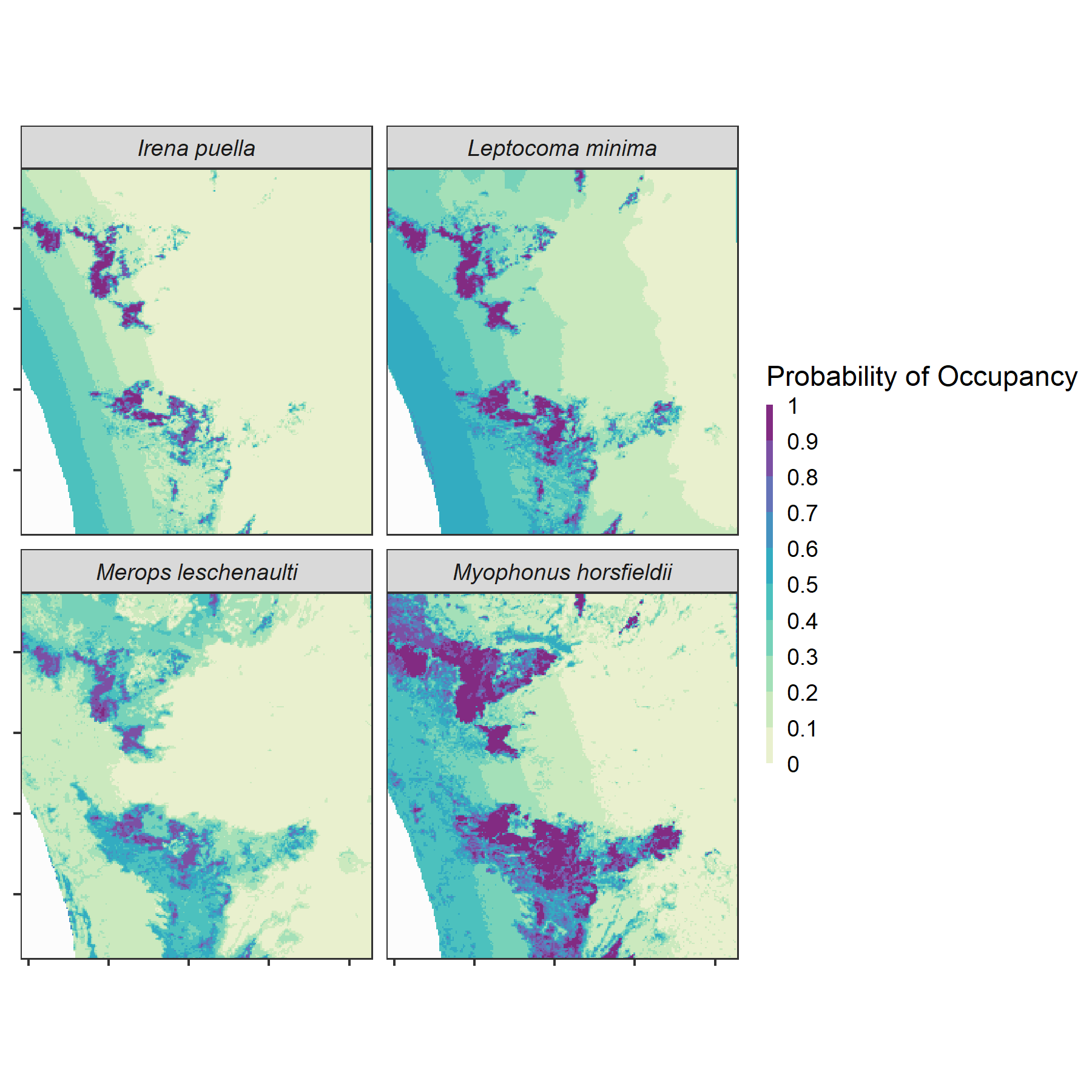
Predicted area of occurrence Predicted area of occurrence for four forest species are shown here. The probability of occupancy of the asian fairy-bluebird Irena puella, the crimson-backed sunbird Leptocoma minima and the chestnut-headed bee-eater Merops leschenaulti is higher across the western slopes and at mid-elevations across our study area. The Malabar whistling-thrush Myophonus horsfieldii has a higher probability of occupancy across mid-elevations throughout the study area examined.

11.7.8 Prepare species occupancy for all species

# multiply coefficients with layers
sp_occu <- map(
  sp_coefs$data,
  .f = function(df) {
    response <- unlist(slice(df, 1), use.names = F) * landscape
    response <- sum(response, na.rm = TRUE) # remove NA layers, i.e., non-sig preds

    # now transform for probability occupancy
    response <- 1 / (1 + exp(-response))
  }
)

# make single stack
sp_occu <- reduce(sp_occu, c)
# assign names
names(sp_occu) <- sp_coefs$scientific_name

# use stars for plotting with ggplot
library(stars)
library(colorspace)

sp_occu <- st_as_stars(sp_occu)

fig_occu_map_all <-
  ggplot() +
  geom_stars(
    data = sp_occu
  ) +
  scale_fill_binned_sequential(
    palette = "Purple-Yellow",
    name = "p(Occu.)",
    rev = T,
    limits = c(0, 1),
    na.value = "grey99",
    breaks = seq(0, 1, 0.1), show.limits = T
  ) +
  facet_wrap(
    ~band,
    labeller = labeller(
      band = function(x) str_replace(x, "\\.", " ")
    )
  ) +
  coord_sf(
    crs = 32643,
    expand = FALSE
  ) +
  theme_test(
    base_size = 8
  ) +
  theme(
    # legend.position = "rg",
    axis.title = element_blank(),
    axis.text = element_blank(),
    legend.key.height = unit(10, "mm"),
    legend.key.width = unit(1, "mm"),
    strip.text = element_text(
      face = "italic"
    ),
    strip.background = element_blank(),
    legend.title = element_text(
      vjust = 1
    )
  )

# save figure
ggsave(
  fig_occu_map_all,
  filename = "figs/fig_occupancy_maps.png",
  width = 16, height = 16
)